This page contains all the MATLAB scripts for the examples presented in DSP Lab 2.

If you are having trouble viewing these MATLAB examples, I recommend using Firefox on a desktop computer or laptop (not mobile device)

MATLAB script for creating Figure 1 and Figure 2 in DSP Lab 2

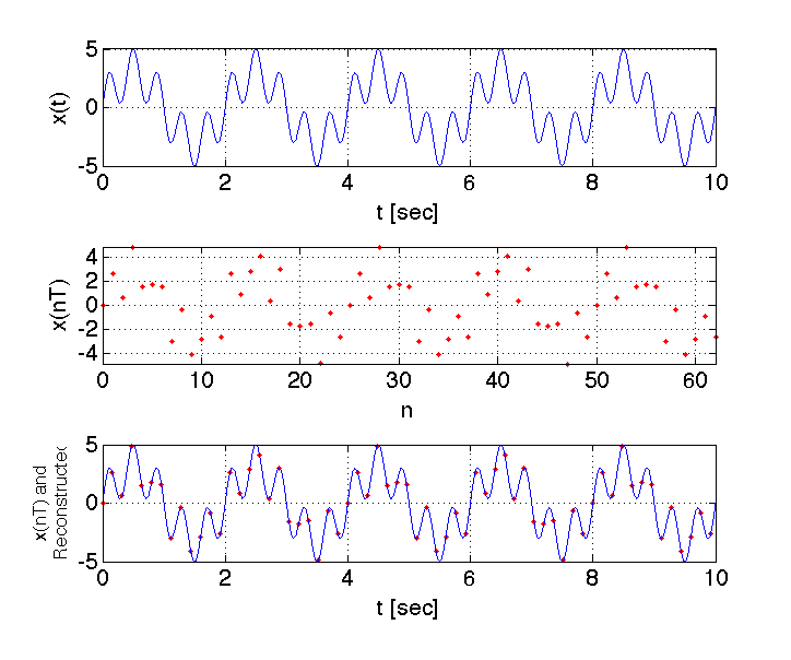
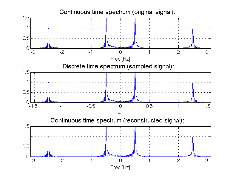
clc;
clear all;
close all;
%%%%%% TIME DOMAIN PLOT (FIGURE 1)
%==================================================
%PLOT THE ORIGINAL CONTINUOUS TIME DOMAIN SIGNAL x(t)
%==================================================
f1=1/2;  % frequency f1 in Hz
f2=2.5; % frequency f2 in Hz
fs=1000*f2; %sampling frequency. When plotting the time-domain signal we
%take a very high sampling frequency so that the plotted signal
%will appear continuous to the eye.
t=[0:1/fs:10]; %plot 10 seconds
x=3*sin(2*pi*f1*t)+2*sin(2*pi*f2*t); %time domain signal we are
%sampling.
figure('color',[1 1 1]); %Note: Open new figure. Set background color to
%white.
subplot(3,1,1)
h=plot(t,x);
ylabel('x(t)','FontSize',16)
xlabel('t [sec]','FontSize',16)
axis tight
set(gca,'FontSize',16)
grid on
%==================================================
%Sampling at fs=2.5*fmax=2.5*f2
%==================================================
fs = 2.5*f2; % Sampling Frequency
t_samp=[0:1/fs:10]; %plot 10 seconds.
xs = 3*sin(2*pi*f1*t_samp)+2*sin(2*pi*f2*t_samp); %create sampled signal
subplot(3,1,2);
n_vector=t_samp*fs; %sampled index array: n=[0, 1, 2, 3, ...., N]
h=plot(n_vector,xs,'r.','markers',13);
ylabel('x(nT)','FontSize',16)
xlabel('n','FontSize',16)
axis tight
set(gca,'FontSize',16)
grid on
%==================================================
%Reconsturcted signal
%==================================================
xr=x; %reconstructed signal xr(t) equals the original continuous time domain
%signal x(t) because the sampling condition is met
subplot(3,1,3)
h=plot(t_samp,xs,'r.',t,x,'b','markers',13);
str = {'x(nT) and', 'Reconstructed'};
ylabel(str,'FontSize',13)
xlabel('t [sec]','FontSize',16)
axis tight
set(gca,'FontSize',16)
grid on
%
%%%%%% FREQUENCY DOMAIN PLOT (FIGURE 2)
%==================================================
%PLOT SPECTRUM OF ORIGINAL CONTINUOUS TIME DOMAIN SIGNAL x(t)
%==================================================
figure('color',[1 1 1]); %Note: Open new figure. Set background color to
%white
fs=1000*f2; %sampling frequency. When creating the continuous time-domain
%signal we take a very high sampling frequency so that the plotted signal
%will appear continuous to the eye.
t=[0:1/fs:30]; %plot 30 seconds (for frequency domain plots, you want to
%simulate many periods of the signal so that your frequency domain plots
%have a high resolution (frequency tones appear "sharp")
x=3*sin(2*pi*f1*t)+2*sin(2*pi*f2*t); %time-domain signal
N=2^20; %good general value for FFT (Leave this number alone for Lab 1)
y=fft(x,N); %compute FFT! There is a lot going on "behind the scenes" with
%this one line of code.
z=fftshift(y); %Move the zero-frequency component to the center of the
%array. This is used for finding the double-sided spectrum (as opposed to
%the single-sided spectrum).
f_vec=[0:1:N-1]*fs/N-fs/2; %Create frequency vector (this is an array of
%numbers. Each number corresponds to a discrete point in frequency in which we
%shall evaluate and plot the function.)
amplitude_spectrum=abs(z)/length(x); %Extract the amplitude of the spectrum
%Here we also apply a scaling factor of 1/length(x), so that the amplitude
%of the FFT at a frequency component equals that of the ideal double-sided
%spectrum.
subplot(3,1,1)
plot(f_vec,amplitude_spectrum);
set(gca,'FontSize',13) %set font size of axis tick labels to 15
xlabel('Freq [Hz]','fontsize',13)
title('Continuous time spectrum (original signal):','fontsize',17)
%ylabel('Spectrum of x(t)','fontsize',13)
grid on
%axis tight
xlim([-6.25/2,6.25/2])
%==================================================
%Sampling at fs=2.5*fmax=2.5*f2
%==================================================
fs = 2.5*f2; % Sampling Frequency
t_samp=[0:1/fs:30];
xs = 3*sin(2*pi*f1*t_samp)+2*sin(2*pi*f2*t_samp); %create sampled signal
N=2^20;
y=fft(xs,N);
z=fftshift(y);
amplitude_spectrum=abs(z)/length(xs);
w_vec=[0:1:N-1]*pi/N-pi/2; %create discrete time frequency (omega hat)
subplot(3,1,2)
plot(w_vec,amplitude_spectrum);
set(gca,'FontSize',13) %set font size of axis tick labels to 15
xlabel(['$$\hat{\omega}$$'],'Interpreter','Latex','fontsize',13)
str = {'Spectrum of', 'sampled signal'};
%ylabel(str,'fontsize',13)
title('Discrete time spectrum (sampled signal):','fontsize',17)
grid on
%axis tight
xlim([-pi/2,pi/2])
%==================================================
%Reconsturcted signal
%==================================================
f_vec=w_vec*fs/pi; %Scale frequency axis
subplot(3,1,3)
plot(f_vec,amplitude_spectrum);
grid on
xlim([-fs/2,fs/2])
xlabel('Freq [Hz]','fontsize',13)
title('Continuous time spectrum (reconstructed signal):','fontsize',17)
set(gca,'FontSize',13) %set font size of axis tick labels to 15

pic
pic

MATLAB script for creating Figure 3 and Figure 4 in DSP Lab 2

clc;
clear all;
close all;
%%%%%% TIME DOMAIN PLOT (FIGURE 3)
%==================================================
%PLOT THE ORIGINAL CONTINUOUS TIME DOMAIN SIGNAL x(t)
%==================================================
f1=1/2;  % frequency f1 in Hz
f2=2.5; % frequency f2 in Hz
fs=1000*f2; %sampling frequency. When plotting the time-domain signal we
%take a very high sampling frequency so that the plotted signal
%will appear continuous to the eye.
t=[0:1/fs:10]; %plot 10 seconds
x=3*sin(2*pi*f1*t)+2*sin(2*pi*f2*t); %time domain signal we are
%sampling.
figure('color',[1 1 1]); %Note: Open new figure. Set background color to
%white.
subplot(4,1,1)
h=plot(t,x);
ylabel('x(t)','FontSize',16)
xlabel('t [sec]','FontSize',16)
axis tight
set(gca,'FontSize',16)
grid on
%==================================================
%Sampling at fs = 1 Hz
%==================================================
fs = 1; % Sampling Frequency
t_samp=[0:1/fs:10]; %plot 10 seconds.
xs = 3*sin(2*pi*f1*t_samp)+2*sin(2*pi*f2*t_samp); %create sampled signal
subplot(4,1,2);
n_vector=t_samp*fs; %sampled index array: n=[0, 1, 2, 3, ...., N]
h=plot(n_vector,xs,'r.','markers',15);
ylabel('x(nT)','FontSize',16)
xlabel('n','FontSize',16)
axis([0 10 -5 5])
set(gca,'FontSize',16)
grid on
%==================================================
%Original and sampled
%==================================================
subplot(4,1,3);
n_vector=t_samp*fs; %sampled index array: n=[0, 1, 2, 3, ...., N]
h=plot(t,x,n_vector/fs,xs,'r.','markers',15);
str = {'x(t) and', 'x(nT)'};
ylabel(str,'FontSize',16)
xlabel('t [sec]','FontSize',16)
axis([0 10 -5 5])
set(gca,'FontSize',16)
grid on
%==================================================
%Reconstructed signal
%==================================================
xr=5*sin(2*pi*0.5*t); %reconstructed signal xr(t) does NOT equal
%the original continuous time domain
%signal x(t) because the sampling condition is not met.
%The reconstructed signal is the corrupted by aliasing.
subplot(4,1,4)
h=plot(t_samp,xs,'r.',t,xr,'b','markers',15);
str = {'x(nT) and', 'Reconstructed'};
ylabel(str,'FontSize',13)
xlabel('t [sec]','FontSize',16)
axis tight
set(gca,'FontSize',16)
grid on
%%%%%% FREQUENCY DOMAIN PLOT (FIGURE 4)
%==================================================
%PLOT SPECTRUM OF ORIGINAL CONTINUOUS TIME DOMAIN SIGNAL x(t)
%==================================================
figure('color',[1 1 1]); %Note: Open new figure. Set background color to
%white
fs=1000*f2; %sampling frequency. When creating the continuous time-domain
%signal we take a very high sampling frequency so that the plotted signal
%will appear continuous to the eye.
t=[0:1/fs:30]; %plot 30 seconds (for frequency domain plots, you want to
%simulate many periods of the signal so that your frequency domain plots
%have a high resolution (frequency tones appear "sharp")
x=3*sin(2*pi*f1*t)+2*sin(2*pi*f2*t); %time-domain signal
N=2^20; %good general value for FFT (Leave this number alone for Lab 1)
y=fft(x,N); %compute FFT! There is a lot going on "behind the scenes" with
%this one line of code.
z=fftshift(y); %Move the zero-frequency component to the center of the
%array. This is used for finding the double-sided spectrum (as opposed to
%the single-sided spectrum).
f_vec=[0:1:N-1]*fs/N-fs/2; %Create frequency vector (this is an array of
%numbers. Each number corresponds to a discrete point in frequency in which we
%shall evaluate and plot the function.)
amplitude_spectrum=abs(z)/length(x); %Extract the amplitude of the spectrum
%Here we also apply a scaling factor of 1/length(x), so that the amplitude
%of the FFT at a frequency component equals that of the ideal double-sided
%spectrum.
subplot(3,1,1)
plot(f_vec,amplitude_spectrum);
set(gca,'FontSize',13) %set font size of axis tick labels to 15
xlabel('Freq [Hz]','fontsize',13)
title('Continuous time spectrum (original signal):','fontsize',17)
%ylabel('Spectrum of x(t)','fontsize',13)
grid on
%axis tight
xlim([-6.25/2,6.25/2])
%==================================================
%Sampling at fs = 1 Hz
%==================================================
fs = .99; % Sampling Frequency
%Note: I set sample rate to 0.99 instead of exactly 1 because,
%when fs = 1 (exacly) the result is very noisey, since the FFT is
%processing a signal which is essentially constant. Changing the
%sampling rate to something very close to 1 (but not exactly 1) fixes
%this problem.  Due to this "fix", however, the precise amplitude of the
%spectrum is not correct, but the general shape of the
%spectrum is correct (i.e. we see a peak at f = plus/minus 0.5 Hz).
t_samp=[0:1/fs:30];
xs = 3*sin(2*pi*f1*t_samp)+2*sin(2*pi*f2*t_samp); %create sampled signal
N=2^20;
y=fft(xs,N);
z=fftshift(y);
amplitude_spectrum=abs(z)/length(xs);
w_vec=[0:1:N-1]*pi/N-pi/2; %create discrete time frequency (omega hat)
subplot(3,1,2)
plot(w_vec,amplitude_spectrum);
set(gca,'FontSize',13) %set font size of axis tick labels to 15
xlabel(['$$\hat{\omega}$$'],'Interpreter','Latex','fontsize',13)
str = {'Spectrum of', 'sampled signal'};
%ylabel(str,'fontsize',13)
title('Discrete time spectrum (sampled signal):','fontsize',17)
grid on
%axis tight
xlim([-pi/2,pi/2])
%==================================================
%Reconstructed signal
%==================================================
f_vec=w_vec*fs/pi; %Scale frequency axis
subplot(3,1,3)
plot(f_vec,amplitude_spectrum);
grid on
xlim([-fs/2,fs/2])
xlabel('Freq [Hz]','fontsize',13)
title('Continuous time spectrum (reconstructed signal):','fontsize',17)
set(gca,'FontSize',13) %set font size of axis tick labels to 15

pic
pic