This lab was developed based upon Reference [1].
Introduction - Sampling and aliasing
An analog-to-digital converter (ADC) converts an analog signal to a digital form.
An ADC produces a stream of binary numbers from analog
signals by taking the samples of the analog signal and digitizing the amplitude at these
discrete times.
Prior to the ADC conversion, an analog filter called the prefilter or antialiasing
filter is applied to the analog signal in order to deal with an effect known as
aliasing.
Aliasing causes multiple continuous time signals
to yield the exact same sampled discrete time signal.
In this lab we focus our attention in the process of sampling and how to avoid the problem
of aliasing. During sampling, an analog signal \(x_a(t)\) is periodically measured
every \(T_s\) seconds:
\begin{equation}
t=nT_s, \quad n = 0,1,2,...
\end{equation}
where \(T_s\) is called the sampling period, and is the fixed time interval between samples
(here we assume a uniform sampling rate that
does not change with time.)
The inverse of \(T_s\) is called the sampling frequency, that is,
the samples per second:
\begin{equation}
f_s=1/T_s.
\end{equation}
When sampling an analog signal we must sample fast enough (i.e. be sure \(f_s\) is sufficiently high),
so that the samples are a good representation of the original analog signal.
If the sampling frequency \(f_s\) is not fast enough then too much information is lost,
and it becomes impossible to reconstruct our original analog signal using a digital-to-analog converter (DAC).
However, if you do sample fast enough, then, theoretically, it is possible to exactly reconstruct the original signal.
Sampling theorem: For accurate representation of signal \(x_a(t)\) by its time samples
\(x[nT]\), two conditions must be met: 1) The signal \(x_a(t)\) must be bandlimited, that is, its
frequency content (spectrum) must be limited to contain frequencies up to some maximum frequency \(f_{max}\)
and no frequencies beyond that, and 2) the sampling rate \(f_s\) must be chosen to be at least
twice the maximum frequency \(f_{max}\), that is
\begin{equation}
f_s \geq 2f_{max}.
\end{equation}
According to the sampling theorem, before sampling we must make sure the signal is
bandlimited (this is the function of the analog prefilter) and that the sampling frequency is
at least twice the maximum frequency.
The traditional Nyquist sampling theorem presented above is true for real-valued
(i.e. not complex), lowpass (i.e. baseband) signals. For complex lowpass signals,
the sampling theorem states that the ultimate minimum sampling rate to avoid
aliasing is actually \(f_s = B\), where \(B\) is the double-sided bandwidth.
For bandpass signals, things get even more interesting. You can subsample (i.e. sample
below the Nyquist rate) to achieve frequency translation to lower frequencies and
recover the original signal. See Reference [2] for more details.
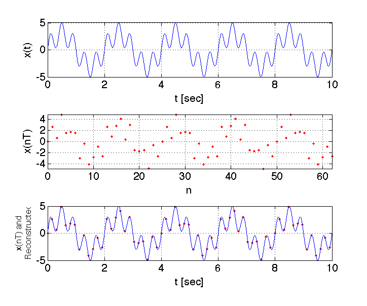
Example 1 - Sampling higher than Nyquist rate
Consider the following continuous time signal:
\begin{equation}
x_a(t)=3\sin(2\pi 0.5t)+2\sin(2\pi 2.5t)
\end{equation}
The signal contains two frequency components at \(f_1\ = 0.5 Hz\) and
\(f_2\ = 2.5 Hz\).
We explore the effect of aliasing by sampling \(x_a(t)\) at \(f_s\ = 2.5f_{max} = 6.25 Hz\).
This sampling frequency meets the sampling theorem requirement. In MATLAB we explore both time-domain
and frequency domains by making the following plots:
- Time domain plots
- The original time signal \(x_a(t)\)
- The sampled signal \(x[n]\) (discrete time signal) with \(f_s=2.5f_{max}=6.25 Hz\)
- The sampled signal superimposed on top of the reconstructed continuous time-signal
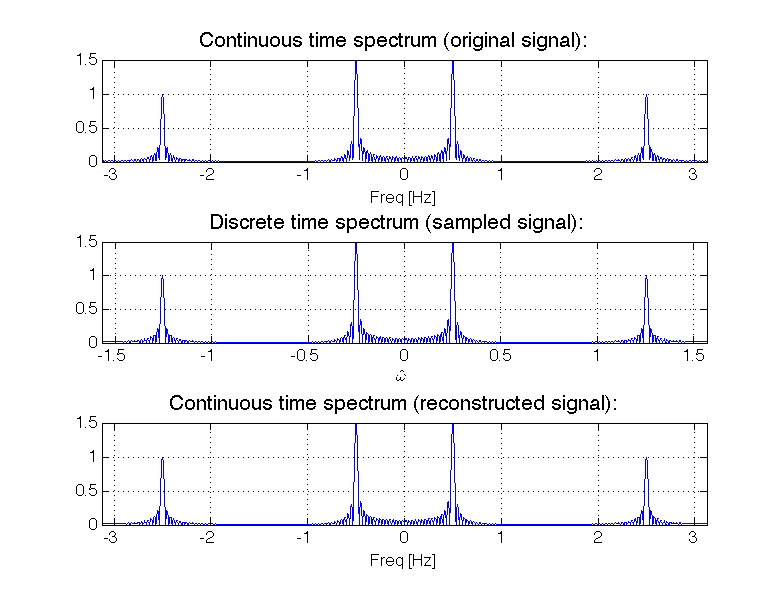
- Frequency domain plots (computed using MATLAB's FFT function)
- The (double-sided) amplitude spectrum of the orignal time domain signal.
- The amplitude spectrum of the sampled signal.
- The amplitude spectrum of the reconstructed continuous time-signal.
Note that the reconstructed time-domain signal is equal to the original time-domain signal, because the sampling
theorem is met. The MATLAB script used to generate this example is
available
here.
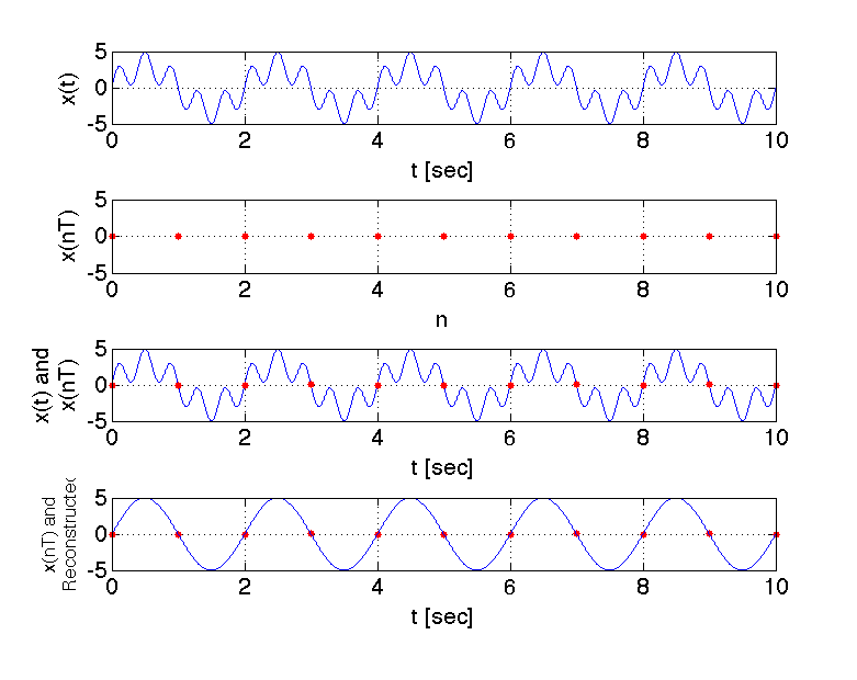
Example 2 - Sampling lower than Nyquist rate
Consider the same continuous time signal as in Example 1:
\begin{equation}
x_a(t)=3\sin(2\pi 0.5t)+2\sin(2\pi 2.5t)
\end{equation}
The signal contains two frequency components at \(f_1\ = 0.5 Hz\) and
\(f_2\ = 2.5 Hz\).
We explore the effect of aliasing by sampling \(x_a(t)\) at \(f_s\ = 1 Hz\).
This sampling frequency does not meet the sampling theorem requirement. In MATLAB we explore both time-domain
and frequency domains by making the following plots:
- Time domain plots
- The original time signal \(x_a(t)\)
- The sampled signal \(x[n]\) (discrete time signal) with \(f_s=f_{max}/2.5=1 Hz\)
- The sampled signal superimposed on top of the original continuous time-signal
- The sampled signal superimposed on top of the reconstructed continuous time-signal
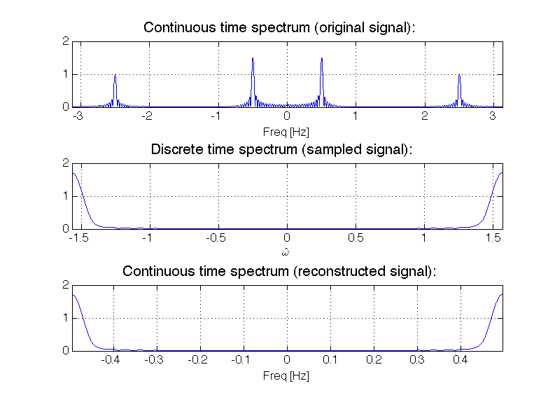
- Frequency domain plots (computed using MATLAB's FFT function)
- The (double-sided) amplitude spectrum of the orignal time domain signal.
- The amplitude spectrum of the sampled signal.
- The amplitude spectrum of the reconstructed continuous time-signal.
Note that the reconstructed time-domain signal is
not equal to the original time-domain signal, because the sampling
theorem is not met. The reconstructed signal is:
\begin{equation}
x_r(t)=3\sin(2\pi 0.5t)+2\sin(2\pi 0.5t) =5\sin(2\pi 0.5t)
\end{equation}
The above equation results because a 0.5 Hz sinusoid is an alias of a 2.5 Hz sinusoid. The MATLAB script used to generate this example is
available
here.
Tasks
Report guidelines
For the lab report, you will create a PowerPoint presentation (or use a similar presentation program), save it as a PDF, and
submit it on-line according to the instructions given in class.
All submitted Matlab code should be well organized and commented with clear comments for easy readability.
All submitted plots should be easy to see and well-labeled.
You are to work independently.
This is not a team assignment.
Feel free to help your fellow classmates understand principles and concepts, but please do not
share your work.
This lab involves generating many plots using MATLAB's subplot
function. This will likely result in figures which are "squashed" together. To unsquash the images, please
manually stretch (resize) the figure window before placing the figures in your presentation.
Your presentation will have 11 slides. Please include a slide number in the footer of each slide. To earn full credit your presentation must
contain the slides in the order asked for in this lab. If you miss a slide, please leave a blank slide in its place so that you have
still have exactly 11 slides total. Your first slide should be:
- Slide 1: Title slide with your name, student ID number, date, lab name, class number/title.
Sampling higher than Nyquist rate
Consider a continuous time domain signal
\begin{equation}
x_a(t)=2\cos(2\pi 0.5t)+\sin(2\pi 1.5t)+\cos(2\pi 2.5t)+1.5\cos(2\pi 3.5t)
\end{equation}
- Suppose we sample \(x_a(t)\) with a sampling frequency \(f_s = 10f_{max}\).
Create a 3-by-1 plot like Example 1 where you plot the original continuous
time signal \(x_a(t)\), the sampled discrete time signal \(x[n]\), and
the sampled discrete time signal superimposed over the reconstructed signal.
Present your plot and your MATLAB code in
Slides 2 - 5. Please program MATLAB to display
your name as the title of the plot.
(e.g. The MATLAB command would be something like: title('Jane Doe').)
Sampling lower than Nyquist rate
- Consider the continuous time signal \(x_a(t)\) expressed in Equation (7).
Suppose we sample \(x_a(t)\) with a sampling frequency \(f_s = f_{max}\).
Create a 4-by-1 plot like Example 2 where you plot the original continuous
time signal \(x_a(t)\), the sampled discrete time signal \(x[n]\),
the sampled discrete time signal superimposed over the original continuous
time signal,
and
the sampled discrete time signal superimposed over the reconstructed signal.
Present your plot in
Slide 6.
Please program MATLAB to display
your name as the title of the plot.
(e.g. The MATLAB command would be something like: title('Jane Doe').)
Anti-aliasing filter
-
Consider the continuous time signal \(x_a(t)\) expressed in Equation (7).
Consider again a sampling frequency \(f_s = f_{max}\).
Suppose you first process \(x_a(t)\) with an ideal anti-aliasing low-pass
prefilter and then sample the signal. What is the signal after the anti-aliasing
low-pass prefilter? Present your expression in Slide 7.
Create a 4-by-1 plot where you plot the original continuous
time signal \(x_a(t)\), the continuous time signal after it has been processed by the prefilter,
the sampled discrete time signal \(x[n]\), and
the sampled discrete time signal superimposed over the reconstructed signal.
Present your plot
Slide 8.
Please program MATLAB to display
your name as the title of the plot.
(e.g. The MATLAB command would be something like: title('Jane Doe').)
The Atari (wrap-around) Effect
- Consider a continuous time domain complex signal
\begin{equation}
x_a(t)=e^{j2\pi10t}
\end{equation}
Create a 4-by-1 plot where you plot the double-sided spectrum of the sampled
signal for the following sampling frequencies: \(f_s = 25 Hz\), \(f_s = 21 Hz\),
\(f_s = 19 Hz\), \(f_s = 15 Hz\).
Present your plot in
Slide 9.
Please program MATLAB to display
your name as the title of the plot.
(e.g. The MATLAB command would be something like: title('Jane Doe').)
When creating your signal, sample your signal for a total of 10 seconds or more (this
large sampling window will result in "sharp" spectral peaks). For your plot make sure
to set axis tight.
- Consider a continuous time domain signal
\begin{equation}
x_a(t)=\cos(2\pi10t)
\end{equation}
Create a 4-by-1 plot where you plot the double-sided spectrum of the sampled
signal for the following sampling frequencies: \(f_s = 25 Hz\), \(f_s = 21 Hz\),
\(f_s = 19 Hz\), \(f_s = 15 Hz\).
Present your plot in
Slide 10.
Please program MATLAB to display
your name as the title of the plot.
(e.g. The MATLAB command would be something like: title('Jane Doe').)
When creating your signal, sample your signal for a total of 10 seconds or more (this
large sampling window will result in "sharp" spectral peaks). For your plot make sure
to set axis tight.
-
In Slide 11 explain what is meant by the Atari (wrap-around)
effect in terms of sampling and aliasing.