clc
clear all
f=[0:1:20]; %frequency axis
A=0*f; %initialize amplitude spectrum by setting all values to zero
A(11) = 1; %amplitude at f = 10 Hz is equal to 1
A(16) = 0.5; %amkplitude at f = 15 Hz is equal to 0.5
stem(f,A,'filled') %create stem plot. Fill in the circles
set(gca,'FontSize',18) %set font size of axis tick labels to 18
xlabel('Frequency [Hz]','fontsize',18)
ylabel('Amplitude','fontsize',18);
title('Amplitude spectra','fontsize',18);
grid on
set(gcf,'color','w'); %set background color from grey (default) to white

clc
clear all
f=[-20:1:20]; %frequency axis
A=0*f; %initialize amplitude spectrum by setting all values to zero
index1 = find(f==-10,1); %find the index of array f corresponding to f = -10
index2 = find(f==10,1); %find the index of array f corresponding to f = +10
index3 = find(f==-15,1); %find the index of array f corresponding to f = -15
index4 = find(f==15,1); %find the index of array f corresponding to f = +15
A(index1) = 0.5; %amplitude at f = -10 Hz is equal to 0.5
A(index2) = 0.5; %amplitude at f = 10 Hz is equal to 0.5
A(index3) = 0.25; %amplitude at f = -15 Hz is equal to 0.25
A(index4) = 0.25; %amplitude at f = +15 Hz is equal to 0.25
stem(f,A,'filled') %create stem plot. Fill in the circles
set(gca,'FontSize',18) %set font size of axis tick labels to 18
xlabel('Frequency [Hz]','fontsize',18)
ylabel('Amplitude','fontsize',18);
title('Amplitude spectra','fontsize',18);
grid on
set(gcf,'color','w'); %set background color from grey (default) to white

clc
clear all2
A = 2; %Amplitude of cosine
f0=100; %Frequency of cosine [Hz]
phi = 0; %Relative phase angle of cosine [radians]
T=1/f0; %period of cosine
fs=100*100; %Sampling frequency
Ts=1/fs; %sampling period
t_begin = 0; %Start plotting at this time
t_end = 3*T; %End plotting at this time
t_vec=[t_begin:Ts:t_end]; %Create time vector (this is an array of numbers.
%Each number corresponds to a discrete point in time in which we shall
%evaluate and plot the function.)
x=A*cos(2*pi*f0*t_vec+phi); %Create our sampled analog cosine signal
plot(t_vec,x,'LineWidth',2) %Plot. Set line width to 2
set(gca,'FontSize',18) %set font size of axis tick labels to 18
xlabel('Time [seconds]','fontsize',18)
ylabel('Amplitude','fontsize',18)
Title('Plot of Acos(2 \pi ft), A = 2 and f = 100 Hz','fontsize',18)
grid on
set(gcf,'color','w'); %set background color from grey (default) to white

clc
clear all
f0=3; %Frequency of simulated signal [Hz]
T=1/f0; %period of signal [s]
fs=f0*50; %Sampling frequency [Hz]
Ts=1/fs; %sampling period [s]
t_begin = 0; %Start plotting at this time
t_end = 3*T; %End plotting at this time
t_vec=[t_begin:Ts:t_end]; %Create time vector (this is an array of numbers.
%Each number corresponds to a discrete point in time in which we shall
%evaluate and plot the signals.)
theta=2*pi*f0*t_vec; %this is the argument in the complex exponential function
x1=exp(j*theta); %Create our sampled analog signal 1
x2=cos(theta)+j*sin(theta); %Create our sampled analog signal 2
plot(t_vec,real(x1),t_vec,real(x2),'b.',t_vec,imag(x1),t_vec,imag(x2),'g.') %Plot.
set(gca,'FontSize',18) %set font size of axis tick labels to 18
xlabel('Time [seconds]','fontsize',18)
ylabel('Amplitude','fontsize',18)
%Title('Plot of Acos(2 \pi ft), A = 2 and f = 100 Hz','fontsize',18)
Title('Demonstration of Euler''s Equation','fontsize',18)
grid on
box off
axis tight
set(gcf,'color','w'); %set background color from grey (default) to white
legend('Re(e^{j\omegat})','cos(\omegat)','Im(e^{j\omegat})','sin(\omegat)')

clc
clear all
close all
f0=3; %fundamental frequency of square wave.
fs=3*60000; %sample frequency (much higher than fundamental frequency).
t=[0:1/fs:1]; %Create array of discrete points in time in which we shall
%evaluate and plot the function.) Here we plot from t = 0 seconds to t = 1
%second.
%Below we create the first five terms in the Fourier series
x0=1/2; %DC component
n=1; %fundamental frequency (first harmonic)
x1=(2/pi)*sin((2*n-1)*2*pi*f0*t)/(2*n-1);
n=2; %(second harmonic)
x2=(2/pi)*sin((2*n-1)*2*pi*f0*t)/(2*n-1);
n=3; %(third harmonic)
x3=(2/pi)*sin((2*n-1)*2*pi*f0*t)/(2*n-1);
n=4; %(forth harmonic)
x4=(2/pi)*sin((2*n-1)*2*pi*f0*t)/(2*n-1);
figure(1)
figure('color', [1,1,1]) %this is another way of setting the background
%to be white.
subplot(4,1,1)
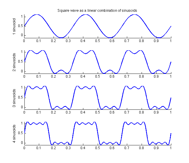
plot(t,x0+x1,'LineWidth',2); box off; axis tight;
title('Square wave as a linear combination of sinusoids')
ylabel('1 sinusoid')
subplot(4,1,2)
plot(t,x0+x1+x2,'LineWidth',2); box off; axis tight;
ylabel('2 sinusoids')
subplot(4,1,3)
plot(t,x0+x1+x2+x3,'LineWidth',2); box off; axis tight;
ylabel('3 sinusoids')
figure(2)
subplot(4,1,4)
plot(t,x0+x1+x2+x3+x4,'LineWidth',2); box off; axis tight;
ylabel('4 sinusoids')
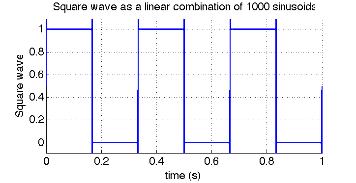
%Let's now add 1000 sinusoids!
N=1000; %number of sinusoids
x=1/2; %inialize the series with the DC term.
for n=1:N
    y=(2/pi)*sin((2*n-1)*2*pi*f0*t)/(2*n-1); %sinusoid corresponding to index k.
    x=x+y; %compute the sum
end
figure('color',[1,1,1]');
plot(t,x,'LineWidth',2);
xlabel('time (s)','fontsize',18); ylabel('Square wave','fontsize',18);
title('Square wave as a linear combination of 1000 sinusoids','fontsize',18)
set(gca,'FontSize',18)
grid on
box off
axis tight

clc;
clear all;
clf;
f0=15; %Highest frequency component of signal [Hz].
fs=3*f0; %Sampling frequency [Hz].
T=1/f0; %period of cosine
Ts=1/fs; %sampling period
t_begin = 0; %Start plotting at this time
t_end = 20*T; %End plotting at this time
t_vec=[t_begin:Ts:t_end]; %Create time vector (this is an array of numbers.
%Each number corresponds to a discrete point in time in which we shall
%evaluate and plot the function.)
x=cos(2*pi*10*t_vec)+0.5*cos(2*pi*15*t_vec); %Create our sampled analog cosine signal
%Compute (fast) Fourier Transform of our analog signal to find it's
%spectrum:
N=2^16; %good general value for FFT (Leave this number alone for Lab 1)
y=fft(x,N); %compute FFT! There is a lot going on "behind the scenes" with
%this one line of code.
z=fftshift(y); %Move the zero-frequency component to the center of the
%array. This is used for finding the double-sided spectrum (as opposed to
%the single-sided spectrum).
f_vec=[0:1:N-1]*fs/N-fs/2; %Create frequency vector (this is an array of
%numbers. Each number corresponds to a discrete point in frequency in which we
%shall evaluate and plot the function.)
amplitude_spectrum=abs(z)/length(x); %Extract the amplitude of the spectrum
%Here we also apply a scaling factor of 1/length(x), so that the amplitude
%of the FFT at a frequency component equals that of the ideal double-sided
%spectrum.
plot(f_vec,amplitude_spectrum);
set(gca,'FontSize',18) %set font size of axis tick labels to 18
xlabel('Frequency [Hz]','fontsize',18)
ylabel('Amplitude','fontsize',18)
Title('Amplitude spectra','fontsize',18)
grid on
set(gcf,'color','w'); %set background color from grey (default) to white
axis tight