How to capture raw IQ data from a RTL-SDR dongle and FM demodulate with MATLAB

Prepared by Dr. Aaron Scher [email protected] Oregon Institute of Technology Back to Aaron's home page.

Capture data and import into MATLAB

1. The first goal is to identify an interesting frequency band to capture. For now I'll capture some of the FM broadcast band. To do this I open GQRX by typing the following in the Terminal:

   gqrx

   The GQRX SDR applications runs. I set the sample rate to be 2500000 samples/second, which equates to a 2.5 MHz bandwidth, and I set the center frequency to 100.122 MHz. Below is a screenshot of the GQRX application. You can identify the radio stations as the "bumps" in the spectrum that rise above the noise floor. We identify the following FM stations (Portland, Oregon):
   1. KUPL 98.7 FM
   2. KWJJ 99.5 FM plus 99.5-1 HD1 and 99.5-2 HD2
   3. KRKT 99.9 FM
   4. KKRZ 100.3 FM plus 100.3-1 HD1 and 100.3-2 HD2
   5. KQRZ 100.7 FM
   6. KXL 101.1 FM

   

2. Now I use the rtl-sdr IQ recorder utility to capture some data. First I close GQRX to free up the RTL dongle. Next, to see the options and default settings for the rtl-sdr utility, I type the following at the Terminal window:

   rtl_sdr

   The Terminal window returns the following:

   rtl_sdr, an I/Q recorder for RTL2832 based DVB-T receivers Usage: [-f frequency_to_tune_to [Hz] [-s samplerate (default: 2048000 Hz)] [-d device_index (default: 0)] [-g gain (default: 0 for auto)] [-p ppm_error (default: 0)] [-b output_block_size (default: 16 * 16384)] [-n number of samples to read (default: 0, infinite)] [-S force sync output (default: async)] filename (a '-' dumps samples to stdout)

   Now, suppose I want to capture 10 seconds worth of data, with a center frequency of 100.122 MHz and a gain of 40 dB. If I set the sample rate to 2500000 samples/sec (which, equates to 2.5 MHz bandwidth) then I will need to capture 25000000 samples (250000000 [samples]/ (2500000 [samples/sec]) = 10 [sec]), and I type the following command at the Terminal:

   rtl_sdr -f 100122000 -g 40 -s 2500000 -n 25000000 FMcapture1.dat

   The Terminal responds with

   Found 1 device(s): Realtek, RTL2838UHIDIR, SN: 00000001 Using device 0: Generic RTL2832U OEM Found Rafael Micro R820T tuner Exact sample rate is: 2500000.107620 Hz Sampling at 2500000 S/s. Tuned to 100122000 Hz. Tuner gain set to 40.20 dB. Reading samples in async mode...

   The raw, captured IQ data is saved in a file called FMcapture1.dat, which is stored in my home directory by default. You can download the file by clicking here:

   FMcapature1.dat

   The raw, captured IQ data is 8 bit unsigned data. Each I and Q value varies from 0 to 255 (since, 00000000₂ = 0 and 11111111₂ = 255). To get from the unsigned (0 to 255) range we need to subtract 127.5 from each I and Q value, which results in a new range from -127.5 to +127.5. Then the complex data is simply y = I + jQ. We perform this using Matlab by applying the following custom function loadFile, which is presented below. You can download this function by clicking here.

   function y = loadFile(filename) % y = loadFile(filename) % % reads complex samples from the rtlsdr file % fid = fopen(filename,'rb'); y = fread(fid,'uint8=>double'); y = y-127.5; y = y(1:2:end) + i*y(2:2:end);

   To make things easier, I add the desktop to the search path in Matlab and save the data file to my desktop. Below I show my MATLAB session for loading the data and checking out the size of the variable:

   >>y=loadFile('FMcapture1.dat'); >>size(y) ans =     25000000         1

   You can see that the captured signal y contains 25000000 (complex) samples as expected. This is a large array! Given a sampling frequency of (approximately) 2500000 Hz, this corresponds to a 10 second sample as expected.

   Plot the spectrum

   Suppose I want to plot the spectrum of the first 0.002 seconds-long "piece" of the full 10 second-long sample. Given that there are 2500000 samples/sec, 0.002 seconds of data contains 5000 samples. I choose to plot the spectrum using the MATLAB function freqz by typing the following in the MATLAB workspace:

   >>y=loadFile('FMcapture1.dat'); >>freqz(y(1:5000),1,[-4E6:.01E6:4E6],2.5E6); >>set(gcf,'color','white');

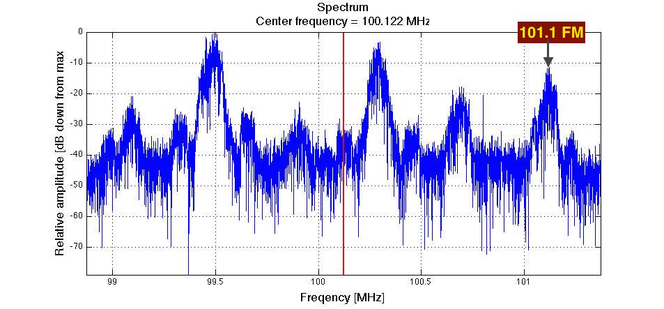
   Here, I purposely set the frequency span from -4 MHz to 4 MHz to see outside the principle alias frequency range. Below is a plot of the magnitude of the spectrum. For clarity I identify all the 101.1 FM aliases. Some important points to note about the spectrum are:
   1. The spectrum is centered at 0 Hz (DC). In our minds, we map 0 Hz to the known center frequency (100.122 MHz).
   2. The spectrum is periodic with a period equal to the sampling frequency (2.5 MHz).
   3. The figure below explicitly shows numerous aliases of the 101.1 FM station (I randomly chose to show 101.1 FM out of the six stations in our bandwidth). So, which one is the "true" 101.1 FM? There is no real answer to this question, since all aliases are indistinguishable (all aliases cary the same information). However, by convention (and for convenience) we will focus on the principle alias band only (frequencies between -1.25 MHz to +1.25 MHz). There is only one alias of the 101.1 FM station that falls within the principle frequency band, and the center frequency of this "principle alias" is at 101.1 MHz - 100.122 MHz = 0.9780 MHz.
   4. Remember that you are looking at the spectrum of a sampled complex IQ signal (I+jQ). When we sample a real signal (such as an ordinary time-domain waveform like a person's voice), the negative frequency part of the spectrum gives no new information, since the spectrum is symmetrical about zero for such a case. When we sample complex signals (like in this example), the spectrum is generally not symmetrical, and negative frequencies contain as much information as positive frequencies - which doubles the amount of total information compared to a sampled real signal. More about negative frequencies, positive frequencies, and complex signals can be found in M. Valkama's presentation Complex Valued Signals and Systems.

   

   To streamline the process of plotting the spectrum, I present below a Matlab function plot_FFT_IQ.m that plots the spectrum of a small segment of data, where the frequency axis is centered at the centered frequency, and only the principle alias frequency band is displayed. A red vertical line is drawn through the center frequency point. You can download the function by clicking here.

   function plot_FFT_IQ(x,n0,nf,fs,f0,title_of_plot) % % plot_FFT_IQ(x,n0,nf) % % Plots the FFT of sampled IQ data % %           x -- input signal %           fs -- sampling frequency [MHz] %           f0 -- center frequency [MHz] %           n0 -- first sample (start time = n0/fs) %           nf -- block size for transform (signal duration = nf/fs) %           title_of_plot--title of plot (string) (optional) % %-This extracts a segment of x starting at n0, of length nf, and plots the FFT. % x_segment=x(n0:(n0+nf-1)); %extracts a small segment of data from signal p=fftshift(fft(x_segment)); %find FFT z = 20*log10(abs(p)/max(abs(p))); %normalize Low_freq=(f0-fs/2); %lowest frequency to plot High_freq=(f0+fs/2); %highest frequency to plot N=length(z); freq=[0:1:N-1]*(fs)/N+Low_freq; plot(freq,z); axis tight xlabel('Freqency [MHz]','FontSize', 14) ylabel('Relative amplitude [dB down from max]','FontSize', 14) grid on set(gcf,'color','white'); if nargin==6     title(title_of_plot,'FontSize', 14) else     title({'Spectrum',['Center frequency = ' num2str(f0) ' MHz'] },'FontSize', 14) end title({'Spectrum',['Center frequency = ' num2str(f0) ' MHz'] },'FontSize', 14) %Add vertical line y1=get(gca,'ylim'); hold on; plot([f0 f0],y1,'r-','linewidth',2); hold off;

   I now apply the plot_FFT_IQ function to plot the spectrum of a 0.002 second segment of the sample, by typing the following into the Matlab command line:

   >> y=loadFile('FMcapture1.dat'); >> plot_FFT_IQ(y,1,.002*2.5E6,2.5,100.122);

   The result is the following plot (I added the station labels):

   

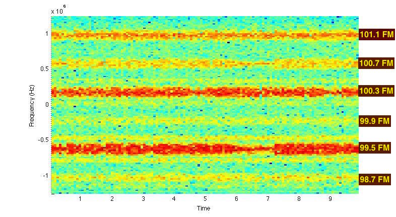
   We can also use MATLAB to plot a spectrogram of the signal. Below I show how to command MATLAB to compute and display the spectrogram of y. Here the signal is divided into sections of length 200000, with 1500 samples of overlap between adjoining sections. The frequency axis is set between -1.25 MHz and +1.25 MHz (principle frequency axis).

   >> y=loadFile('FMcapture1.dat'); >> spectrogram(y,200000,1500,[-1.25E6:.02E6:1.25E6],2.5E6,'yaxis'); >>set(gcf,'color','white');

   The result is the following plot (I added the "101.1 FM" label):

   

   FM demodulate

   Let's FM demodulate the 100.3 FM broadcast. To do this, we first want to center the 100.3 FM station at 0 Hz (DC). Remember, 0 Hz maps to our center frequency (100.122 MHz). The center of the 100.3 MHz FM station is 0.178 MHz above 100.122 MHz. Therefore, we need to frequency down shift our signal by 0.178 MHz to center the 100.3 FM station at 0 Hz (DC). We can do this in MATLAB by multiplying our signal y by a complex exponential, as demonstrated by the following MATLAB commands:

   >> y=loadFile('FMcapture1.dat'); >> y_shifted=y.*transpose(exp(-j*2*pi*0.178E6*[1:1:length(y)]/2.5E6));

   To plot the spectrum (of the first 0.002 seconds of the frequency-shifted signal), we type the following MATLAB command:

   >> plot_FFT_IQ(y_shifted,1,.002*2.5E6,2.5,101.1,'Spectrum of shifted signal'); ;

   This yields the following plot:

   

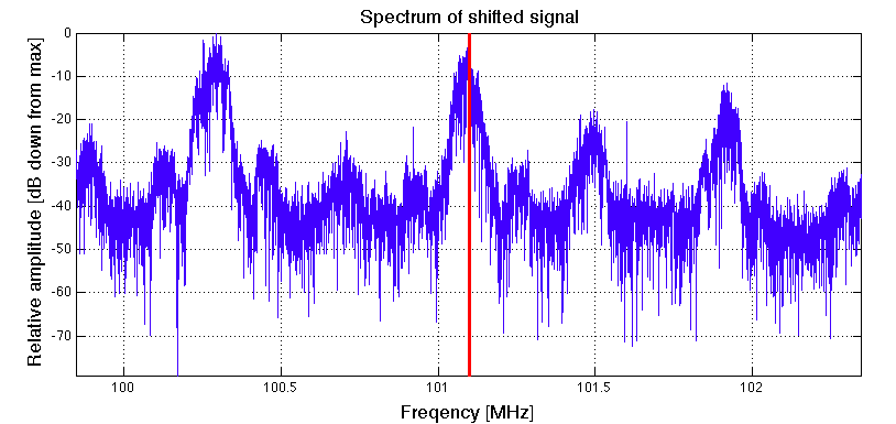
   If you look closely (i.e. zoom in) you will see that the the 100.3 FM station isn't perfectly centered at 0 Hz. This is due to a small frequency offset in the hardware's local oscillator (this offset was there all along). However, the offset is sufficiently small for our purposes, so we don't need to worry about it. The next step is to apply a low pass filter to keep 100.3 FM, but block (i.e. severely attenuate) all the other stations. We are going to use MATLAB's decimate function to achieve this. MATLAB's decimate function is a "two for one special". It first low pass filters the signal to guard against aliasing, and then it reduces the original sampling rate to a lower rate. 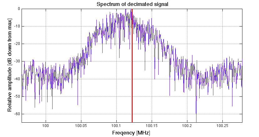We will decimate our original signal by, say, a factor of 8. This yields a new sampling frequency of (2.5 MHz)/8 = 312.5 kHz, and filters out the other stations. To do this, we type the following MATLAB command:

   >> d = decimate(y_shifted,8,'fir');

   Here we saved our decimated signal as the variable d. To plot the spectrum (of the first 0.002 seconds of the decimated signal), we type the following MATLAB command:

   >> plot_FFT_IQ(d,1,.002*2.5E6/8,2.5/8,100.122,'Spectrum of decimated signal');

   This yields the following plot:

   

   A custom function called FM_IQ_Demod for demodulating the FM signal is presented below. You can download the function by clicking here.

   function [y_FM_demodulated] = FM_IQ_Demod(y) %This function demodualtes an FM signal. It is assumed that the FM signal %is complex (i.e. an IQ signal) centered at DC and occupies less than 90% %of total bandwidth. b = firls(30,[0 .9],[0 1],'differentiator'); %design differentiater d=y./abs(y);%normalize the amplitude (i.e. remove amplitude variations) rd=real(d); %real part of normalized siganl. id=imag(d); %imaginary part of normalized signal. y_FM_demodulated=(rd.*conv(id,b,'same')-id.*conv(rd,b,'same'))./(rd.^2+id.^2); %demodulate! end

   I intend to present the theory behind this function at a later time. In the meantime, if you are interested, I used the frequency demodulation algorithm presented in this webpage: DSP Tricks: Frequency demodulation algorithms. There are many ways to demodulate an FM signal. This is just one I picked because it seemed simple enough and yields good results.

   To use the FM_IQ_Demod function and plot the spectrum of the resulting baseband signal, we type the following into the MATLAB workspace:

   >> [y_FM_demodulated] = FM_IQ_Demod(d); %d is the decimated signal >>plot_FFT_IQ(y_FM_demodulated,1,.05*2.5E6/8,2.5/8,0,'Spectrum of demodulated signal');

   The resulting spectrum is plotted below:

   

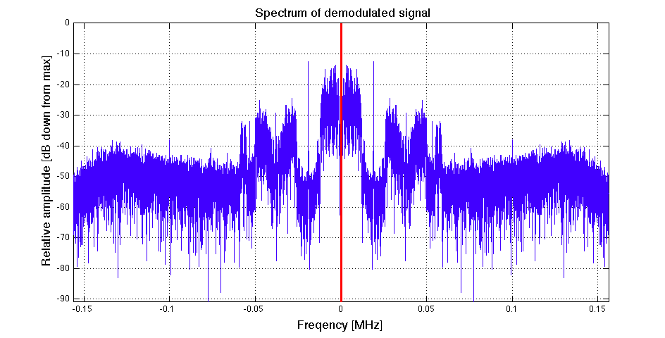
   Note that the demodulated signal is purely real. It is no longer a complex IQ signal. From a spectral point of view, this means the negative frequency side is a conjugate-mirror image of the positive frequency side (you can see this in the picture above). Compare the spectrum above with the "Typical spectrum of composite baseband signal" presented in Wikipedia's page on FM Broadcasting (shown below). You can clearly identify the mono audio channel (left+right), 19kHz stereo pilot, stereo audio channel (left-right), and RBDS signal.

   

   Listen to station in mono

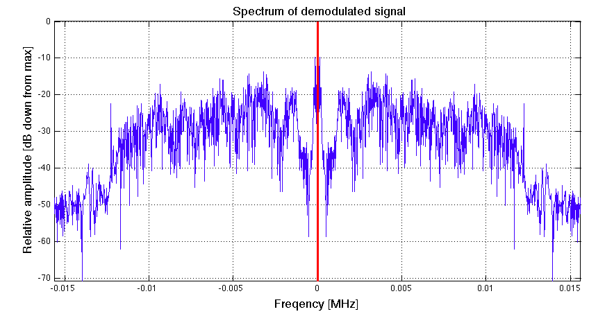
   Now I decimate one more time to bring the sampling rate of the signal within the range of my audio card on my computer.

   >> df = decimate(y_FM_demodulated,10,'fir');

   Here I decimated the sampling rate by 8, which results in a new sampling rate equal to (312.5 kHz)/10 = 31.25 KHz, which is in the range of my sound card while capturing the mono audio channel only. To plot the spectrum of the resulting signal, I type the following into MATLAB:

   >> plot_FFT_IQ(df,1,.05*2.5E6/8/10,2.5/8/10,0,'Spectrum of demodulated signal');

   The spectrum is shown below:

   

   There is only one thing left to do... Listen to the music! I do this by typing the following into MATLAB:

   >> sound(df,2.5E6/8/10);

   If you want to have some fun (i.e. listen to the radio station slowed down), try this:

   >> sound(df,2.5E6/8/10/2);