Introduction

Here I show how to simulate phase locked loops (PLLs) with MATLAB. For more information on PLLs in general I suggest checking out my video Simulating an Analog Phase Locked Loop .

PLL: Type 1

Below is a block diagram of a Type 1 PLL:

Below is the MATLAB program that simulates the above phase locked loop. You can download the m-file by clicking here.

%This program performs a sampled time domain simulation of an
%analog phase locked loop (Type 1 with multiplier and low-pass filter)
%
%Written by Aaron Scher
%
%The reference signal is a simple sinusoid. The output should be a sinusoid
%that tracks the frequency of the reference signal after a certain
%start up time.

%Clear work space variables:
clc
clear all

%User inputs:
f0=1E6; %Frequency of reference signal [Hz]
phase_ref=0; %Phase of reference signal [radians]
fVCO=1.1E6; %free running oscilating frequency of VCO [Hz]
KVCO=.5E6; %Gain of VCO (i.e. voltage to frequency transfer coefficient) [Hz/V]
fs=100E6; %Sampling frequency [Hz]
NF=1000; %Number of samples in simulation
fc=.2E6; %Cut-off frequency of low-pass filter (after the multiplier) [Hz]
filter_coefficient_num=100; %Number of filter coefficeints of low-pass filter

%Start!
b = fir1(filter_coefficient_num,fc/(fs/2)); %design FIR filter coefficients
Ts=1/fs; %sampling period
t_vec=[0:Ts:(NF-1)*Ts]; %time vector

VCO=zeros(1,NF); %initialize VCO signal array
phi=zeros(1,NF); %initialize VCO angle (phi) array
reference=sin(2*pi*f0*t_vec+phase_ref); %input signal

for n=2:NF
    t=(n-2)*Ts; %Current time (start at t = 0 seconds

    error_mult(n)=reference(n)*VCO(n-1);%multiply VCO x Signal input to get raw error signal

    %%%%%%%%%%%%Low pass filter the raw error signal:
    for m=1:length(b)
        if n-m+1>=1
           error_array(m)=error_mult(n-m+1);
        else
           error_array(m)=0;
        end
    end
    error(n)=sum(error_array.*(b));
  %%%%%%%%%%%%%%%%%%%%%%%%%%%%%%
 
    phi(n)=phi(n-1)+2*pi*error(n)*KVCO*Ts; %update the phase of the VCO
    VCO(n)=sin(2*pi*fVCO*t+phi(n)); %compute VCO signal
 
end

%Plot VCO (output) and reference (input) signals:
figure(1)
plot(t_vec,reference,t_vec,VCO)
title('Plot of input and output signals','FontSize',12)
xlabel('time [s]','FontSize',12)
legend('Input','Output')

%Plot error signal:
figure(2)
plot(t_vec,error)
title('Error signal','FontSize',12)
xlabel('time [s]','FontSize',12)

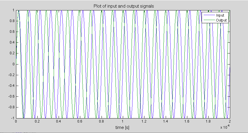
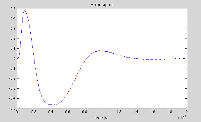
Running the above MATLAB program yields the plots below. At the beginning of the simulation (t = 0 seconds) the VCO is oscillating at its free-running oscillating frequency (1 MHz), while the input signal is fixed at 1.1 MHz (these frequencies are hard coded in the program - you can change these to other values). After the PLL achieves lock, the output signal is locked in frequency to the input signal (i.e. the VCO is oscillating at 1.1 MHz). The error signal is taken at the output of the low-pass-filter. Note that when the PLL achieves lock, the error is a constant. This indicates that the output signal is locked in frequency to the input signal, but there is a phase error. This phase error is characteristic of Type 1 PLLs. If you look carefully, you will see that there is a small ripple in the error signal. This leads phase noise in the output signal.

PLL: Type 2

Below is the block diagram of the PLL:

Below is the MATLAB program that simulates the above phase locked loop. You can download the m-file by clicking here.

%This program performs a sampled time domain simulation of an
%analog phase locked loop (Type 2 with multiplier and low-pass filter)
%
%Written by Aaron Scher
%
%The reference signal is a simple sinusoid. The output should be a sinusoid
%that tracks the frequency of the reference signal after a certain
%start up time.

%Clear work space variables:
clc
clear all

%User inputs:
f0=1E6; %Frequency of reference signal [Hz]
phase_ref=0; %Phase of reference signal [radians]
fVCO=1.1E6; %free running oscilating frequency of VCO [Hz]
KVCO=.5E6; %Gain of VCO (i.e. voltage to frequency transfer coefficient) [Hz/V]
G1=0.4467; %Proportional gain term of PI controller
G2=1.7783e+05; %Integral gain term of PI controller
fs=100E6; %Sampling frequency [Hz]
NF=2000; %Number of samples in simulation
fc=.2E6; %Cut-off frequency of low-pass filter (after the multiplier) [Hz]
filter_coefficient_num=100; %Number of filter coefficeints of low-pass filter

%Start!
b = fir1(filter_coefficient_num,fc/(fs/2)); %design FIR filter coefficients
Ts=1/fs; %sampling period
t_vec=[0:Ts:(NF-1)*Ts]; %time vector

VCO=zeros(1,NF); %initialize VCO signal array
phi=zeros(1,NF); %initialize VCO angle (phi) array
error=zeros(1,NF); %initialize error array
Int_error=zeros(1,NF); %initialize error array
reference=sin(2*pi*f0*t_vec+phase_ref); %input signal

for n=2:NF
    t=(n-2)*Ts; %Current time (start at t = 0 seconds

    error_mult(n)=reference(n)*VCO(n-1);%multiply VCO x Signal input to get raw error signal

    %%%%%%%%%%%%Low pass filter the raw error signal:
    for m=1:length(b)
        if n-m+1>=1
           error_array(m)=error_mult(n-m+1);
        else
           error_array(m)=0;
        end
    end
    error(n)=sum(error_array.*(b));
  %%%%%%%%%%%%%%%%%%%%%%%%%%%%%%
 
  %Process filtered error signal through PI controller:
           Int_error(n)=Int_error(n-1)+G2*error(n)*Ts;
           PI_error(n)=G1*error(n)+Int_error(n);
  %

    phi(n)=phi(n-1)+2*pi*PI_error(n)*KVCO*Ts; %update the phase of the VCO
    VCO(n)=sin(2*pi*fVCO*t+phi(n)); %compute VCO signal
 
end

%Plot VCO (output) and reference (input) signals:
figure(1)
plot(t_vec,reference,t_vec,VCO)
title('Plot of input and output signals','FontSize',12)
xlabel('time [s]','FontSize',12)
legend('Input','Output')

%Plot error signal:
figure(2)
plot(t_vec,error)
title('Error signal','FontSize',12)
xlabel('time [s]','FontSize',12)

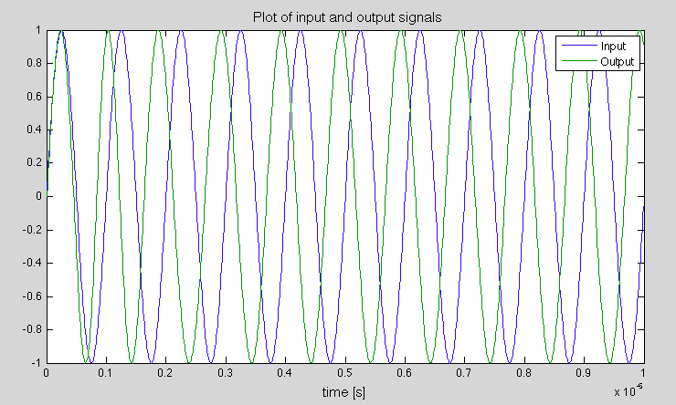
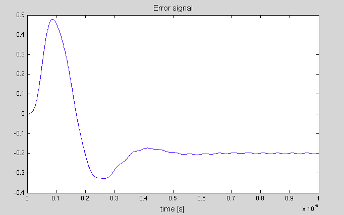
Running the above MATLAB program yields the plots below. At the beginning of the simulation (t = 0 seconds) the VCO is oscillating at its free-running oscillating frequency (1 MHz), while the input signal is fixed at 1.1 MHz (these frequencies are hard coded in the program - you can change these to other values). After the PLL achieves lock, the output signal is locked in frequency and phase to the input signal (both are oscillating at 1.1 MHz with a fixed phase difference of 90 degrees). The error signal at taken as the output of the low-pass-filter. See how the error goes to zero? This indicates that the output signal becomes locked in frequency to the input signal with zero phase error, i.e. the output leads the input by 90 degrees once lock is achieved (we consider 90 degrees phase difference to be "zero phase error"). Zero phase error is characteristic of Type 2 PLLs. If you look carefully, you will see that there is a small ripple in the error signal. This leads to phase noise in the output signal.