For the lab report, you will create a PowerPoint presentation (or use a similar presentation program), save it as a PDF, and
submit it on-line according to the instructions given in class. The presentation should be tutorial in nature; your target audiences are
other engineers and scientists who are interested in learning more about antennas.
Your presentation will have 11 slides. Please include a slide number in the footer of each slide. To earn full credit your presentation must
contain the slides in the order asked for in this lab. If you miss a slide, please leave a blank slide in its place so that you have
still have exactly 11 slides total. Your first two slides should be:
Slide 1: Title slide with our name, student ID number, date, lab name, class number/title.
Slide 2: A team picture or insignia with the names of your teammates.
4. Prelab
Bilco Wifi Cantenna
The Bilco Wifi cantenna is a commercially available 2.4 GHz cantenna from
http://www.bilcowifi.com.
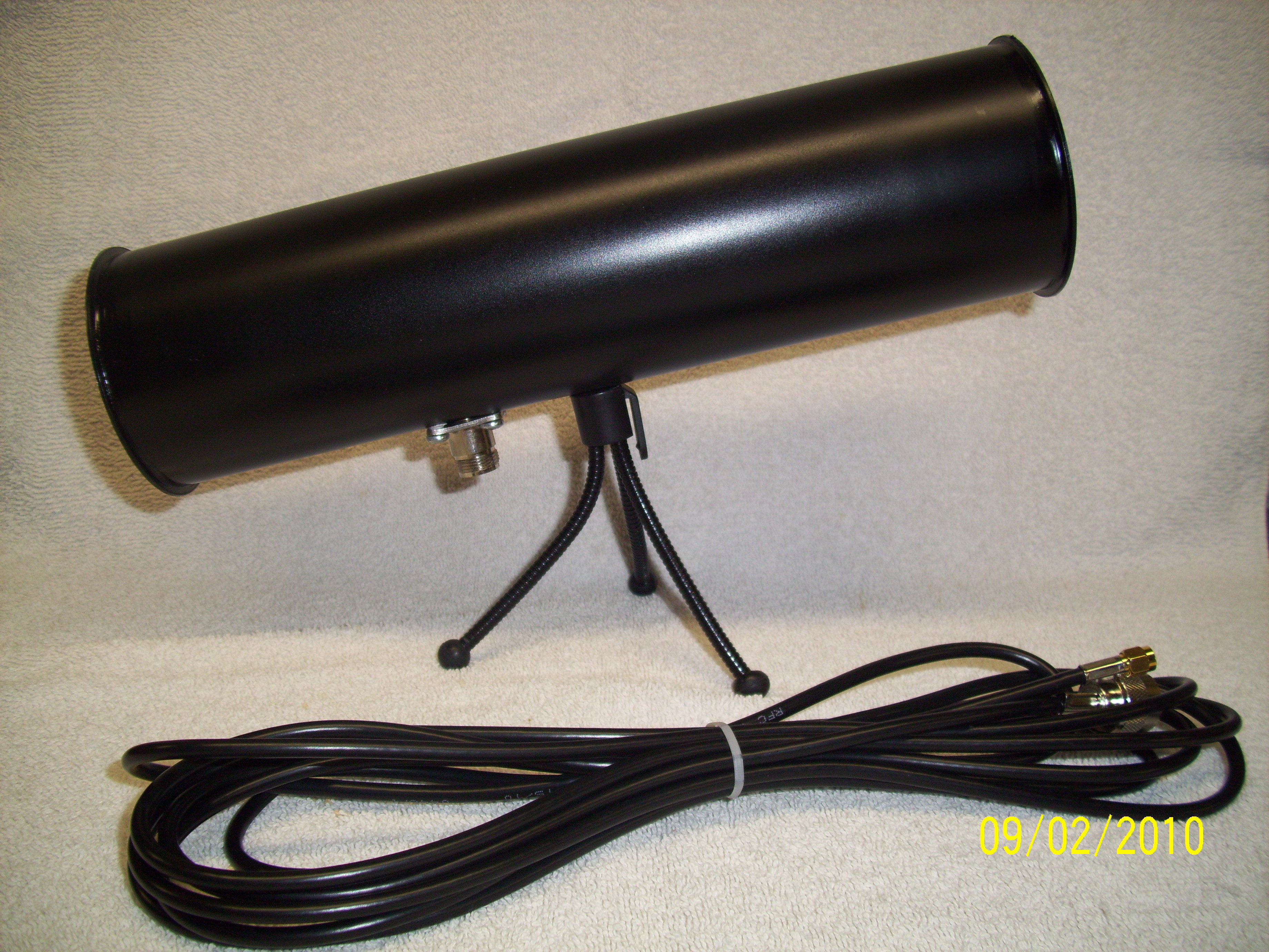
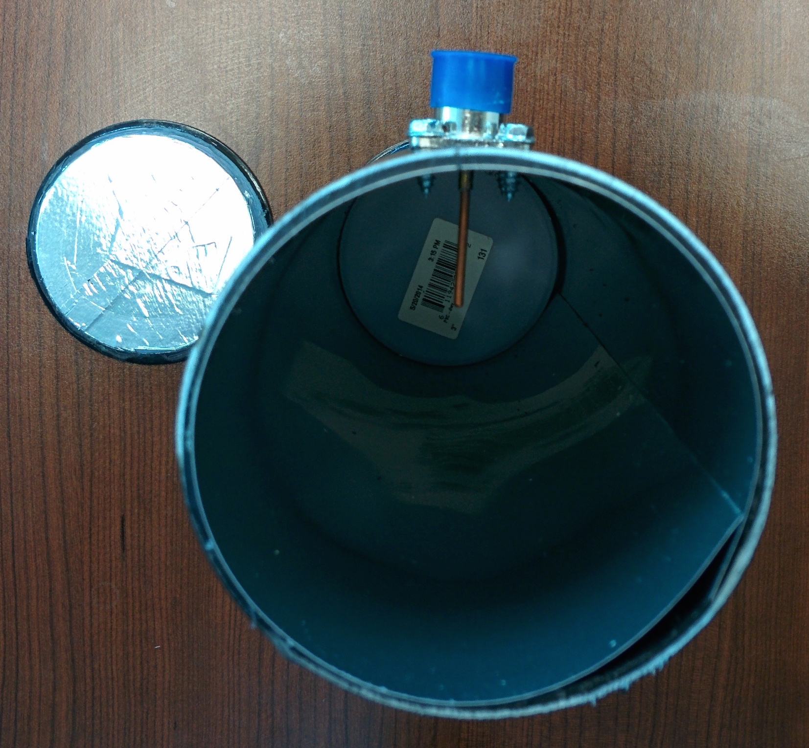
Figures 1 and 2 show pictures of the Bilco WiFi cantenna (12 inch version).
Figure 1. Bilco WiFi cantenna with mount.
Picture from http://www.bilcowifi.com.Figure 2. Bilco WiFi cantenna with end-cap cover removed.
Note that both covers are required to hold shape.
Calculate far-field of cantennas
Calculate the far-field distance of the Bilco Wifi cantenna at the operating frequency.
The criterion for far-field operation that we derived in class is:
Rfar-field =
2D2
λ0
where λ0 is the free-space wavelength at the operating frequency [meters],
and D is the aperture diameter of the can [meters]. The diameter of the Bilco Wifi
antenna is 8.5 cm. Present the value of
Rfar-field for each teammate's cantenna in
Slide 3.
When working through this lab you want to make sure the distance between the receiving and
transmitting antennas is greater than Rfar-field to prevent phase-errors.
Calculate the maximum transmit power permitted for safe operation
The FCC says that the limit for maximum possible exposure (MPE) in our
frequency range of interest is 5 mW/cm2 with an averaging time of 6 minutes.
(see reference.)
To calculate this maximum transmit power, recall that if a source is transmitting power
at Pt with antenna gain G,
the power density Pd in watts per square meters at a distance R
from the source can
be calculated by the following equation:
Pd =
GPt
4πR2
Assume G = 10 dB = 10 and R = 2 inches = 0.051 meters. Calculate and
record the maximum transmit power permitted for safe operation Pt,max
in mW and dBm and present your results in Slide 4.
Make sure your transmit power is at least 3dB below Pt,max.
Procedure
Measure input impedance and VSWR of Bilco WiFi Antenna
Secure Bilco WiFi cantenna to the test platform.
Connect the input of your cantenna to the network analyzer. Use the shortest jumper cable feasible
to reduce cable loss.
Point the antenna in a direction with the fewest obstacles to reduce backscattering.
Set the frequency range on the network analyzer from 2.2 to 2.6 GHz.
Calibrate the network analyzer.
Measure VSWR and input impedance (on the Smith chart). Present screenshots of these
measurements in Slide 5. Is the antenna well-matched?
Measure Antenna Patterns of Bilco WiFi Antenna
Setup your antenna measurement like that illustrated in Figure 3.
Your antennas should be about 2.5 meters apart (L ≈ 2.5 meters.)
Choose a cantenna to serve as your reference antenna, while the other cantenna
will serve as the antenna under test (AUT). The AUT will be secured to a test stand with
a swivel base, while the reference antenna can be secured to a stand with a stationary base.
You will be measuring the pattern of the AUT.
Here are some tips for making accurate measurements
Set the reference antenna and AUT to the same height
Minimize the influence of connector cables by using cable ties.
Make sure the reference antenna and AUT both have the same polarization.
Polarization is defined by the direction of the electric field (E-field) vector.
The E-field vector points in the same direction as the little monopole (wire) in
cavity of the can. To keep things simple, set up both cans so that they are vertically
polarized. This means align the two antennas so that the monopoles in the cavity
(i.e. the driving elements) are both pointing skywards (vertical) as shown in
Figure 3. This setup will be used to measure the pattern in the H-plane. The
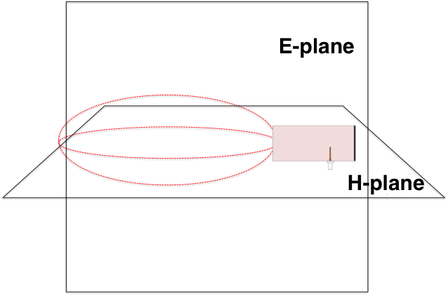
E- and H-planes are illustrated in Figure 4. Note that the driving element
(monopole) is in E-plane and perpendicular to H-plane.
With the reference and AUT setup to make an H-plane measurement like that shown in Figure
3, set the transmit frequency to a 2.4 GHz with a transmit power
Pt < Pt,max, where Pt,max was calculated
in the Prelab.
Rotate the receiver from an azimuth angle of -90° to an azimuth angle of 90° in 10°
steps, recording the received power at each angle. Fill out the second column (labeled
"Vertical position, H-plane (dBm)") in Table 1.
Turn off the transmitter.
Setup the AUT and reference antenna so that their monopoles in the cavity (i.e. the
driving elements) are pointing sideways (horizontal) to measure the antenna pattern cut
in the E-plane. Turn on the transmit power.
Rotate the receiver from an azimuth angle of -90° to an azimuth angle of 90° in 10°
steps, recording the received power at each angle. Fill out the third column (labeled
"Horizontal position, E-plane (dBm)") in Table 1.
Normalize the pattern data for the AUT by the maximum value.
Plot the normalized antenna patterns for the AUT. When you make your graph, correct the angle
so that the maximum angle occurs at 0°. Present your plots of the E-plane and H-plane
in Slide 6 and Slide 7, respectively.
From your plots, determine the half power beamwidth (in the degrees) in the E-plane and H-plane.
Present your results in Slide 8.
Estimate the gain by using the following equation (valid for two identical antennas
perfectly aligned with no reflections from external objects):
where R is the distance between the antennas, Pt is the transmit
power and Pr is the
receive power (maximum value). Present your gain in slide 8.
Figure 3. Setup for
measuring the H-plane antenna pattern.
Figure 4. E and H planes for a vertically polarized cantenna.
Omnidirectional dipole antenna
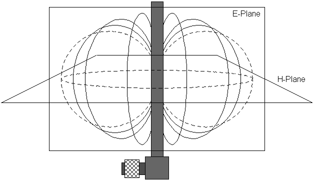
A vertically polarized omnidirectional dipole antenna with the E and H planes is illustrated
in Figure 5. Note that the driving element (dipole) is in E-plane and perpendicular to H-plane.
You will be supplied with a 2.4 GHz omnidirectional antenna like this is for the lab.
This will be your new AUT. Leave the reference antenna the same as before.
Using the network analyzer, measure VSWR and input impedance (on the Smith chart). Present screenshots of these
measurements in Slide 9. Is the antenna well-matched?
Measure the antenna pattern in H-plane and E-plane, like you did for the cantenna.
Normalize the pattern data for the AUT by the maximum value, and present plots of your
patterns in Slide 10 and
Slide 11.
Figure 5. E and H planes for a vertically polarized dipole antenna.
Table 1: Antenna Pattern Measurements (Use this table for both cantenna and omnidirectional dipole antenna measurements.)