To measure and plot the standing wave pattern on a lumped-element transmission line for different loads (open, short, matched, and unmatched resistive loads).
To determine the wavelength of the transmission line from the standing wave ratio and compare this to the theoretical value using the line parameters.
To measure the voltage standing wave ratio (VSWR) for a given load and compare with the expected theoretical value.
2. Equipment
Solderless breadboard (large enough to connect 50 components).
#22 gauge hookup wire for breadboard wiring
Ninteen 0.068 uF capacitors.
A good capacitor to use is the Kemet C322C683K5R5HA (Multilayer Ceramic Capacitors MLCC -
Leaded 50 volts 0.068uF 10% X7R, data sheet).
Can be ordered from
Mouser Electronics here.
Two 0.033 uF capacitors.
A good capacitor to use is the Kemet C322C333J1R5TA (Multilayer Ceramic Capacitor MLCC -
Leaded 100 volts 0.033uF 5% X7R, data sheet).
Can be ordered from
Mouser Electronics here.
Twenty 150 uH inductors. For best results you want low loss inductors. A good inductor to use is the Bourns RLB00712-151KL (data sheet).
Can be ordered from
Mouser Electronics here.
Oscilloscope
Function generator
Wire strippers/cutters.
3. Report guidelines
For the lab report, you will create a PowerPoint presentation (or use a similar presentation program), save it as a PDF, and
submit it on-line according to the instructions given in class. The presentation should be tutorial in nature; your target audiences are
other engineers and scientists who are interested in learning more about circuits and electromagnetism.
Your presentation will have 13 slides. Please include a slide number in the footer of each slide. To earn full credit your presentation must
contain the slides in the order asked for in this lab. If you miss a slide, please leave a blank slide in its place so that you have
still have exactly 13 slides total. Your first two slides should be:
Slide 1: Title slide with your name, student ID number, date, lab name, class number/title, and names of teammates.
4. Introduction
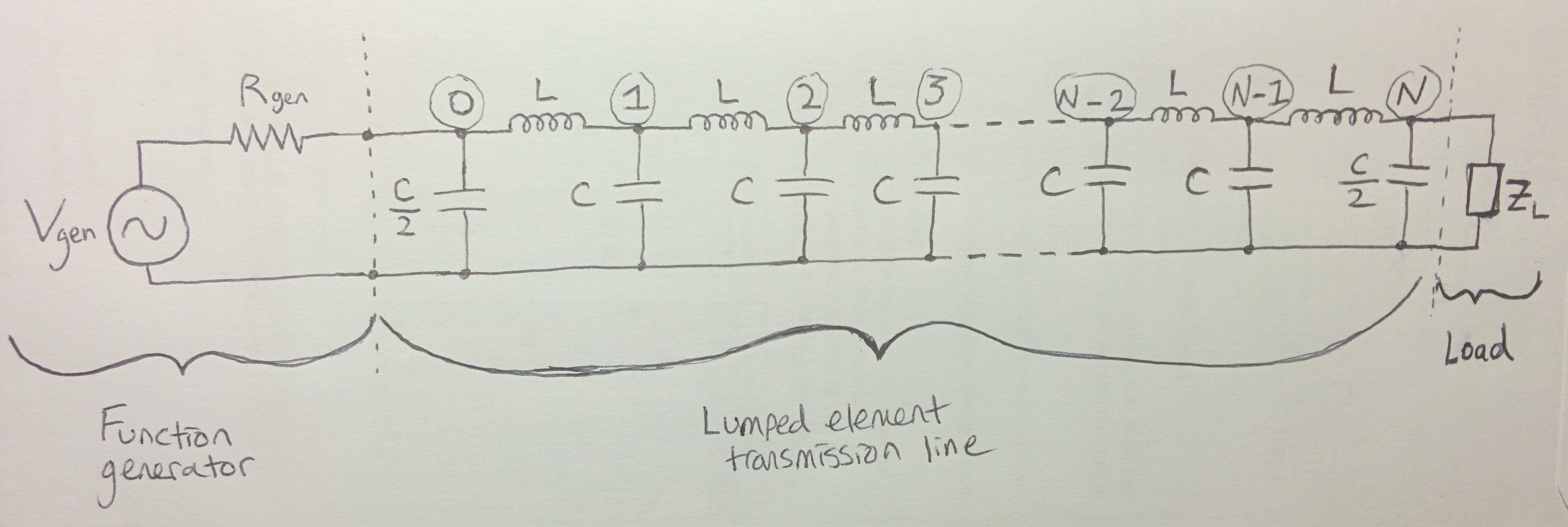
In this lab you are going to construct a lumped-element transmission line like that shown in Figure 1 using a breadboard
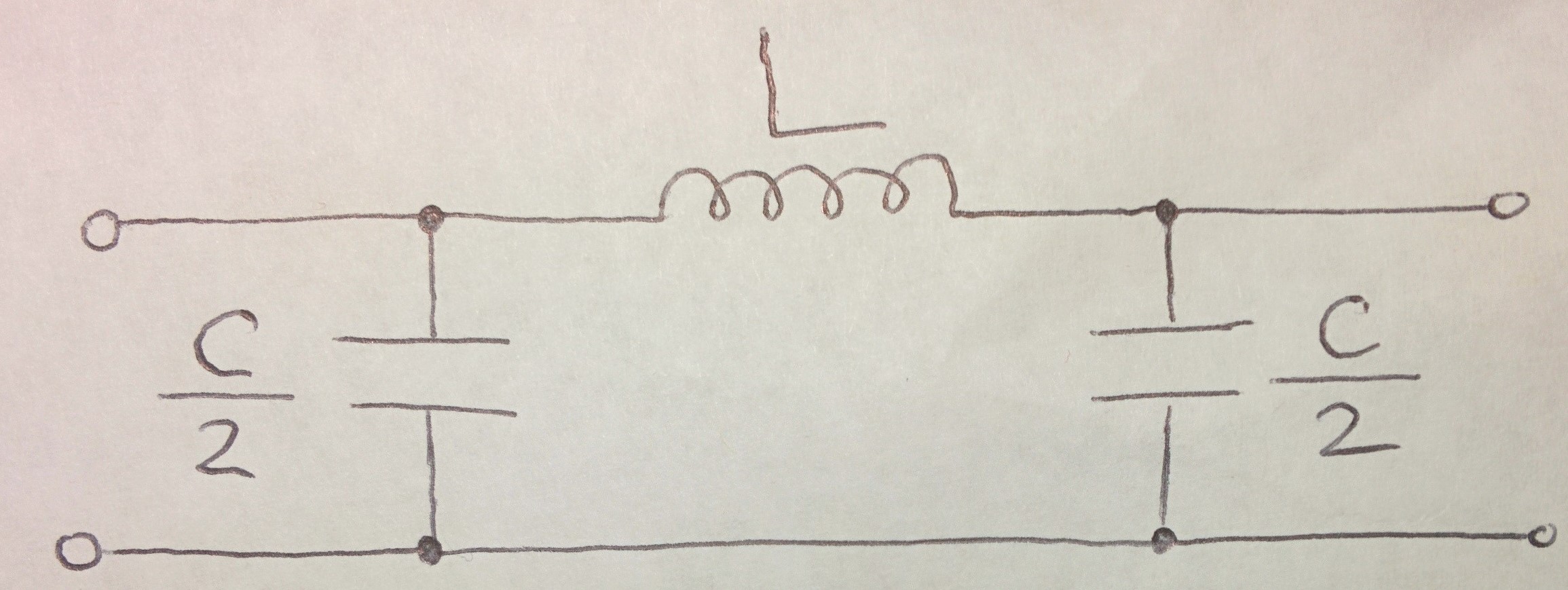
and discrete inductors and capacitors (some people refer to this network as a lumped element delay line). The basic unit cell is shown in Figure 2. A lumped-element transmission line
is a periodic structure composted of a number of these unit cells cascaded together. Note that all capacitors in our
transmission line model share a common ground. Your lumped-element transmission line will be comprised of twenty unit cells (N=20), with
a nominal per-unit-cell inductance L' = 150 uH/cell and per-unit-cell capacitance C'= 0.068 uF/cell.
Hence, your line will contain twenty 150 uH inductors, nineteen 0.068 uF capacitors and two 0.034 uF capacitors (these two "extra" 0.03 4 uF capacitors
appear at the beginning and end of your lumped-element transmission line). For this experiment, the 150 uH inductors and 0.068 uF capacitors were chosen partly because
these are standard valued components
that can easily be found and purchased from popular electronics vendors off the Internet. A 0.034 uF capacitor is not a standard value, and not easily found.
Too make a 0.034 uF capacitor, you can use two 0.068 uF capacitors in series
or use a single 0.033 uF capacitor (0.033 uF is close enough to 0.034 uF for this experiment, especially considering component tolerances).
Figure 1. Lumped-element transmission line connecting a function generator to a load.
Figure 2. Unit cell of the lumped-element transmission line.
In this lab you will measure the voltage between unit cells with respect to ground. By convention,
we assign the index "0" to the node between the source and the first unit cell, as illustrated in Figure 1.
Node 1 is the next node as you move away from the source (i.e. towards the load), and so on. So, if your transmission line is composed of
N unit cells, the last node (i.e. the node between the last unit cell and the load) will have the index "N". Again, in our particular case we have twenty unit
cells, so N=20.
5. Procedure
Calculate characteristic impedance and determine operating frequency
Assuming nominal component values and lossless components, calculate the characteristic impedance using the relationship
Z0=
√ L/C ,
and present this value in Slide 2. The value should be close to 50 Ohms.
It's now time to choose your operating frequency (f). The basic design philosophy here is that
you don't want the equivalent electrical length (phase shift) of a single unit cell to be
too large. This is so you can sample the standing wave along the lumped-element transmission line
with sufficient resolution. Nor do you want the phase shift of a unit cell to be too small;
else you will not observe standing wave effects. We are looking for the goldilocks zone here.
A phase shift of 15 degrees per unit cell is a good compromise (with the added benefit of being a factor
of 90 degrees). Recall the equation for the phase shift per unit cell: β =
2π f√ LC .
Now choose f such that the resulting phase shift per unit cell is 15 degrees (β =π/12 )
Present the value for f (in Hz) in
slide 3.
Building the transmission line
Construct your lumped element transmission line on a breadboard. While a little time consuming, it is recommended that
before you drop down a component,
measure its resistance (to check for damaged components). It is recommended to also measure the inductances of all
inductors and capacitances of all capacitors. This will help you determine and remove "bad apples", and
reduce the need for complicated troubleshooting later. Present the resistance of three randomly chosen inductors
in slide 4.
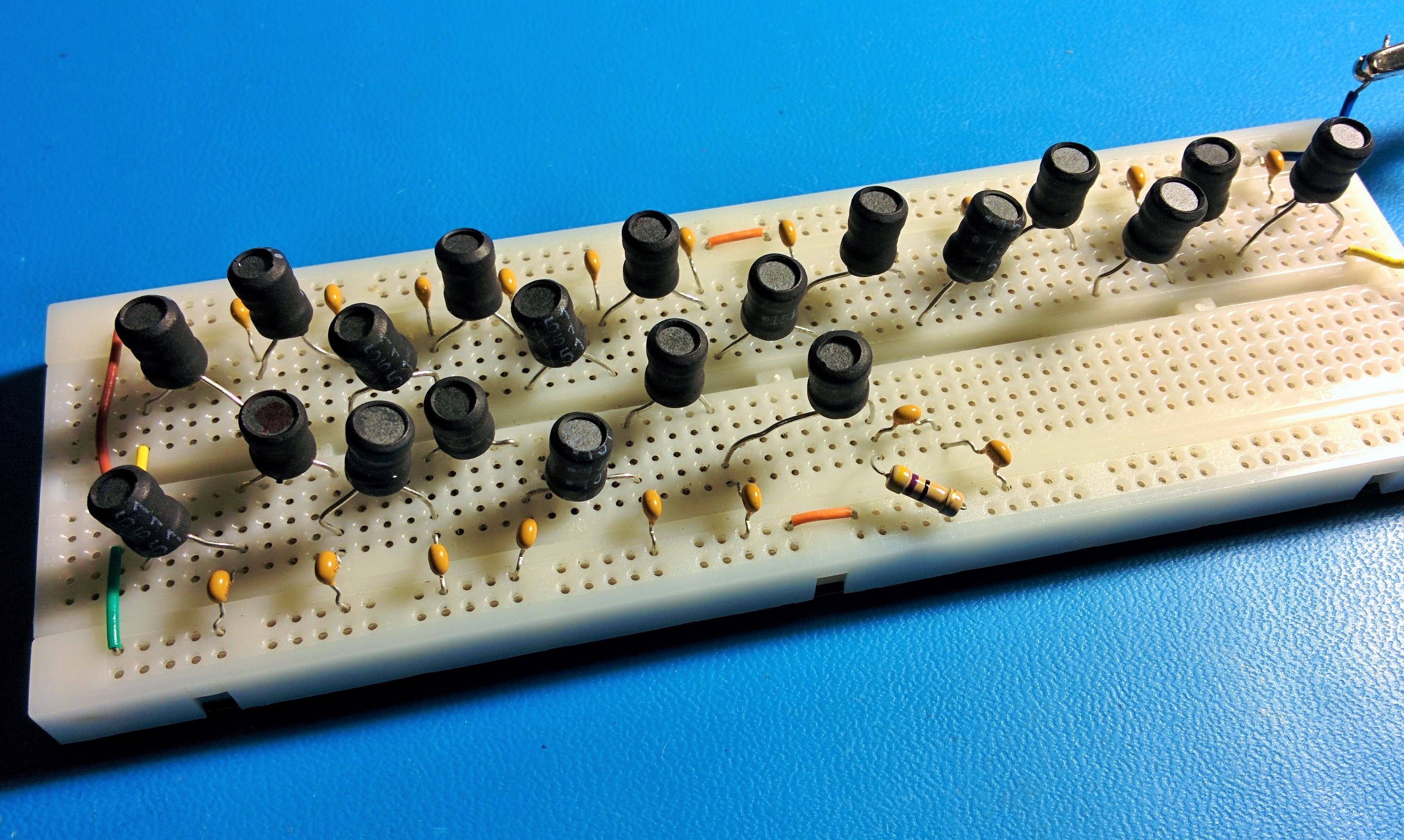
Note that the inductors are unshielded and therefore prone to mutual coupling.
Therefore, when laying out your components, it's important to space your inductors as far apart as possible to reduce this coupling.
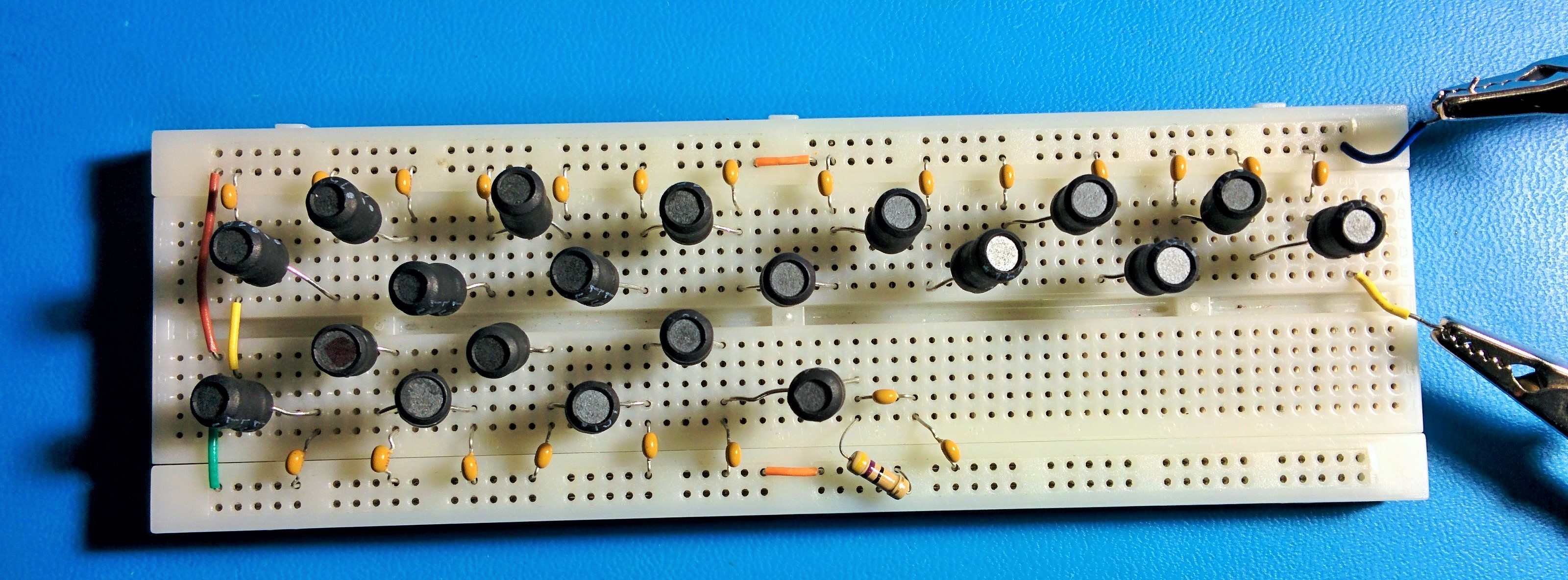
An example layout that worked well for this experiment is shown in Figures 3 and 4. Present a photograph of your
lumped element transmission line in slide 4.
Figure 3. Photograph of lumped-element transmission line .
Figure 4. Top down view of lumped-element transmission line.
Measuring the standing wave pattern
Configure the function generator to generate a sine wave with an amplitude of 5 V. Set the frequency of the generator to the value
you calculated for slide 3. Connect the function generator across the input terminals of your lumped element transmission line.
Your lumped element transmission line is now "live".
Leave the output of your lumped-element transmission line open (do not connect a load).
Using the oscilloscope, confirm that you have a voltage standing wave pattern on the line
by measuring the node voltage amplitudes
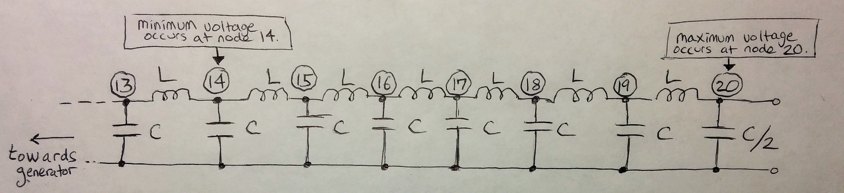
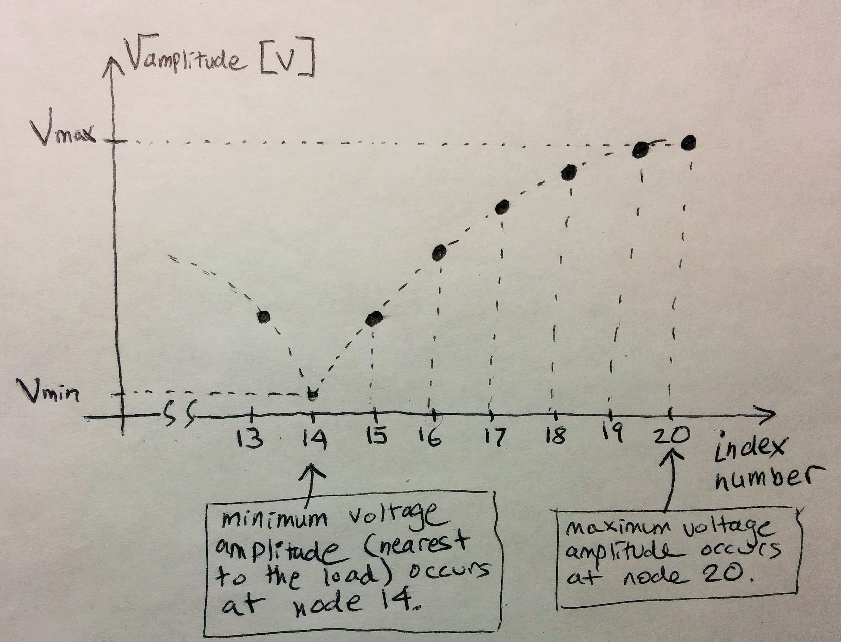
near the load. Figures 5 and 6 illustrate the voltage standing wave pattern near the load end.
Since you set the frequency for a nominal 15 degree phase shift per unit cell, a voltage minimum
occurs at node 14. This node (node 14) is six cells away from the load end; six cells corresponds to
an electrical length of (6 cells)*(15 degrees/cell) = 90 degrees. Because
of component tolerances, however, this may not be exactly 90 degrees. To correct this error,
fine tune the frequency of the function generator
to achieve the lowest possible voltage amplitude at node 14. This (experimentally determined) frequency should be close to that you
calculated in slide 3. Present the new frequency in slide 5.
This will be the frequency you use for the rest of this section.
Figure 5. Lumped element transmission line with an open load.
Figure 6. Plot of standing wave pattern for lumped-element transmission line.
Open load. Plot shows representative voltage amplitudes at nodes 13 - 20.
In slide 6 plot the standing wave pattern for the open load.
To do this, measure the amplitude of the AC voltage at each node (relative to ground) and plot
your values on a graph using a program like Excel or Matlab; the x-axis should be the node number (0 - 20),
and y-axis should be the measured voltage amplitude. If possible, fit an exponentially
decreasing sine wave curve (damped-sine-wave trend line) to your plot. Determine the wavelength
λ (in terms of the number of unit cells) from the standing wave pattern and compare to the ideal, theoretical value
(assuming lossless components with nominal component values). Present your measured λ
and theoretical λ in slide 11. Experimentally measure the VSWR and compare with the ideal, theoretical
value. Present your measured VSWR and theoretical VSWR also in slide 6.
Repeat step 3 in this section for a shorted load and present your results in slide 7.
Repeat step 3 in this section for a matched load (Rload=47 Ohms),and present your results in slide 8.
Also, for the matched load, measure the phase shift difference in degrees between two adjacent nodes (e.g. node 13 and node 14) with the two channels of the oscilloscope.
This phase shift should be near 15 degrees.
Present your results in slide 9.
Pulse propagation
Configure the function generator to generate a square wave with a high state of 5V, a low state of 0V, a frequency of 1 kHz, and a duty cycle of 10%.
Simultaneously measure the voltage amplitude at node 0 and node 20 using the two channels of the oscilloscope.
What is the measured signal delay (in microseconds) of a pulse? What is the theoretical signal delay, calculated
using the nominal component values(L = 150 uH and C= 0.068 uF)? Present the measurements and theoretical calculation/results in slide 10.
Cut-off frequency
The lumped element transmission line is a low pass filter with a cut off frequency
ωc =2/√ LC [1], where the units of ωc are in [radians/second]. This equation assumes a lossless, infinitely long line.
Calculate the theoretical cut-off frequency in [kHz] using this equation with the nominal component values (L = 150 uH and C= 0.068 uF),
and present your result in slide 11.
Connect your lumped element transmission line to a matched load. (Rload=47 Ohms).
Configure the function generator to generate a sine wave with an amplitude of 5 V.
Measure the amplitude of the voltage across node number 20 for a frequency range of f=1 kHz to f=150 kHz, and plot the frequency response.
Do the results agree with the cut-off frequency you calculated in the step above? Present your plot and analysis
in slide 12.
Lumped versus distributed TL
In slides 13 discuss the similarities and differences between lumped transmission lines (constructed out of discrete
components) and distributed transmission lines (such as coax cables and microstrip).
5. References
P. C. Magnusson, V. K. Tripathi, G. C. Alexander, Transmission lines and wave propagation, third edition, CRC Press, 1991.