Back to Aaron's home page.
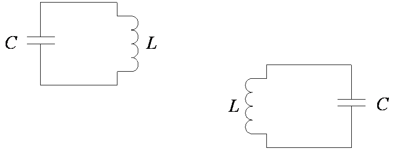
In the world of microwave filter design you hear a lot about coupling:
"coupling matrices", "dual-mode coupling", "cross-coupling", "coupled-lines", "coupling screws", etc.What is all this coupling going on? Generally speaking, the word "coupling" refers to the transfer of energy between two or more physical states or systems. This is a broad definition, and, as such, you could technically say your brain-eye is electromagnetically coupled to the distant stars when you look up on a clear starry night; or, for that matter, that you are coupled to the hand of Van Gough when you enjoy his swirling painting The Starry Night. However, these are examples of one-way coupling. You have no effect on a distant star whatsoever - if it even still exists today - and you certainly have no effect on Van Gough. Ordinarily, people use the word "coupling" to describe systems interacting more intimately with each other, pushing and pulling, exchanging energy back and forth. People generally talk about coupling between oscillators (or resonant systems).
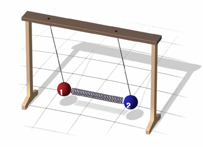
The classic example of coupling between oscillators is two simple mechanical pendula joined by a spring, as illustrated below. If you get one pendulum swinging it will push and pull on the connecting spring giving the second pendulum a small tug. As a result, the second pendulum begins to swing too. If the two pendulums have the same length and mass, the second pendulum continues to swing with ever greater speed as the first pendulum slows down. Eventually, the first pendulum is brought to rest; it has transferred all of its energy to the second pendulum. But now the original situation is exactly reversed, and the first pendulum is positioned to steal back its energy from the second. The process repeats itself over and over, with the energy being passed back and forth like a game of catch, until finally all the energy is dissipated as heat by friction and air resistance. When this happens all mechanical motion ceases.
The electronic analog of the two pendula joined by a spring is a circuit composed of two resonators joined by a coupling element. Energy is coupled in the circuit, not by mechanical springs of course, but by electric and magnetic fields, or a mixture thereof.
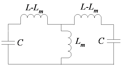
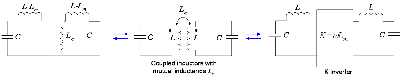
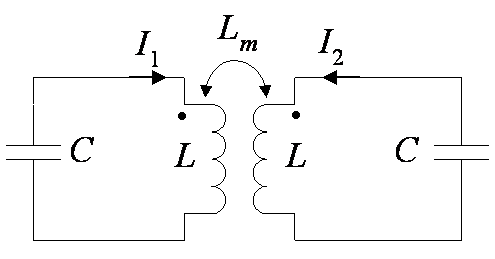
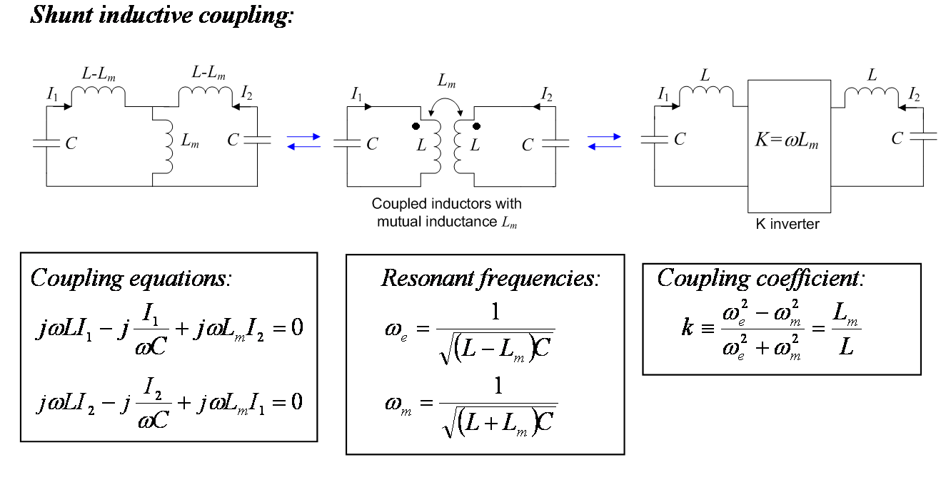
Consider two lossless identical resonators, each with a self inductance L and self capacitance C, existing independently from one another as illustrated in Figure 3 (a). The resonant frequency ω0 of each resonator is related to L and C by the well-known relation ω0 = 1/sqrt(LC). As it stands, the resonators have nothing to do with each other, and are completely decoupled. Now suppose that the resonators are brought together to "share" a little piece of their self-inductance with one another. Suppose this little piece of shared inductance has value Lm (where Lm≤L) as illustrated in Figure 3 (b). In this new situation, the resonators are said to be shunt inductively coupled. Alternate forms of the equivalent circuit are illustrated in Figure 3 (c); these are particularly convenient for design applications.
While each isolated LC resonator supports only one resonant mode individually, the coupled pair as a whole supports two - each with its own resonant frequency. To understand this, consider the form of the coupled pair shown in Figure 4, where we denote the currents in loops 1 and 2 as I1 and I2, respectively. Here we use capital letters for current to remind us that we are dealing with phasor representations in the frequency domain; as usual, lower-case letters are reserved for time domain variables.
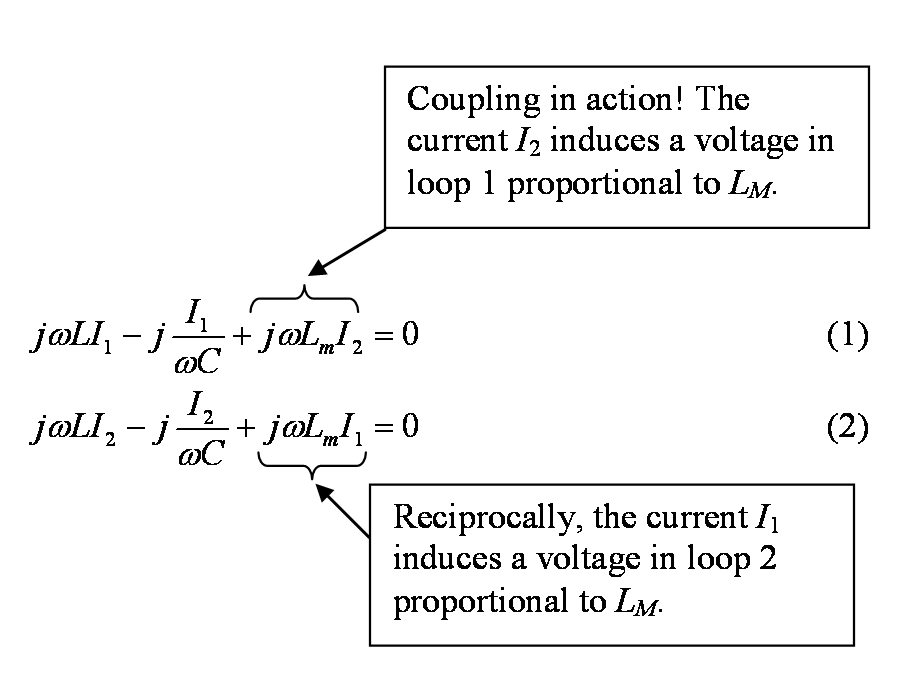
The coupling equations describing this network are:
In matrix form, these equations become:
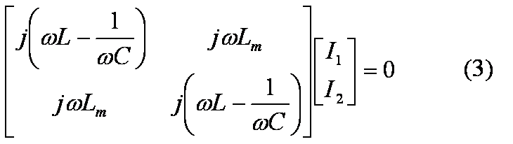
An easy and obvious solution to this matrix equation is simply I1=I2=0. However, this is not a very interesting solution. In fact, a resonant mode is precisely the situation when the currents are not zero. For this to be the case, the 2-by-2 square matrix on the left hand side of Eq (2) must be non-invertible (i.e. it must be singular). Recall from basic linear algebra that a square matrix is singular if and only if its determinant is equal to zero. Singular matrices are rare in the sense that if you pick a random square matrix, it will almost surely not be singular. However, at certain frequencies (which we identify as the resonant frequencies) the 2-by-2 square matrix on the left hand side of Eq (2) will indeed be singular. To find these resonant frequencies, we take the determinant and set it equal to zero.
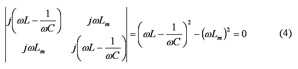
If you crank through the algebra, you will find that this equation has two positive real solutions ωm and ωe, where
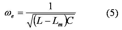
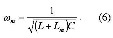
The larger the magnetic coupling Lm, the greater the resonant frequencies ωe and ωm "split away" from that of an uncoupled resonator ω0. On the other hand, in the limit that the coupling is zero, the solutions tend to that of an uncoupled single resonator, i.e. ωe = ωm = ω0 = 1/sqrt(LC) when Lm = 0.
What about the currents I1 and I2 in all of this? If you substitute ω = ωe either into Eq (1) or Eq (2), you will find that I1 = -I2. This means the common current through the "shared" inductance Lm is I1 +I2 = I1 - I1 = 0. From the point of view of the loop current voltages, this condition is equivalent to replacing the symmetry plane between the coupled pair with an electric wall (i.e. a short). The symmetry plane is illustrated in Fig. 5. The subscript "e" in the symbol ωe stands for "electric wall". This mode is referred to as the odd mode. On the other hand, if you substitute ω = ωm into Eq (1) or Eq (2), you will find that I1 = I2. This means the common current through the "shared" inductance Lm is I1 +I2 = 2I1 = 2I2. This condition is equivalent to replacing the symmetry plane with a magnetic wall (i.e. an open). This mode is referred to as the even mode. The subscript "m" in the symbol ωm stands for "magnetic wall".
An important fact to take away from all this is that a coupled pair of resonators forms a composite system with two resonant modes of its own.& The resonant frequencies of these modes are different than that of the uncoupled single resonators. You can say that the original mode has “split” into two. This is a general fact of coupled oscillators: A system composed of N weakly coupled discrete oscillators will in general have N independent states ("state" is a more general term for "mode"). If you increase the number N, then the number of states goes up. Recall the single pendulum swings back and forth with one frequency only - its resonant frequency. Here we have N = 1. On the other hand, consider, say, a guitar string fixed on both ends. Such a structure basically consists of an infinite number of coupled oscillators (i.e. the atoms in the string coupled together by electrostatic forces). As you may know, an ideal vibrating string fixed on both ends has an infinite number of sine waves (i.e. modes or harmonics) it can support. Strum an acoustic guitar to hear some of them.
As it turns out, we are not so much interested in the mutual inductance Lm itself as we are in the ratio of mutual inductance to self inductance: Lm/L. This ratio is a measure of the coupling strength, and is known as the coupling coefficient kM for a pair of synchronously tuned shunt inductive coupled resonators. From energy considerations, it can be shown that the mutual inductance of a pair of coils cannot be greater than the geometric mean of the self-inductances of the coils, i.e.
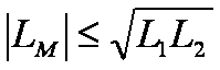
In this manner, the coupling coefficient kM specifies the extent to which LM approaches the upper limit, and satisfies the inequality:
The general coupling coefficient k between any two resonators is defined based on the ratio of the coupled energy to stored energy of the electromagnetic field. The coupling coefficient shows up all the time in filter theory. When people talk about "coupling matrices" of microwave bandpass filters, they really mean a matrix (as in a two-dimensional array of numbers) filled with the coupling coefficients between the various resonators of the filters.
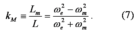
A nice feature of the coupling coefficient is that it can be found from the even and odd mode resonant frequencies, ωm and ωe. From Eqs. (5) and (6) we have:
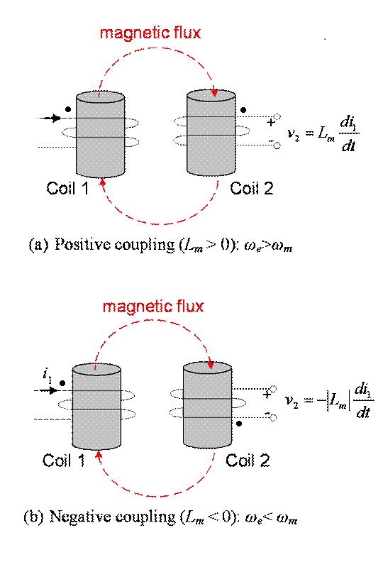
So, by our chosen sign convention, if ωe>ωm then kM is positive, and if ωe<ωm then kM is negative. This sign convention is as arbitrary as assigning a negative electric charge to an electron and a positive electric charge to a proton. But once the sign convention has been made, you must stick with it or else you will lose your way. In order to ensure this sign convention is satisfied every time, we define the general coupling k coefficient to be:
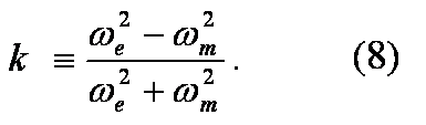
Equation (8) satisfies the strict definition of k given (see Microstrip Filters for RF/Microwave Applications by Hong and Lancaster, Wiley, 2001). This is a powerful equation that can be used to experimentally or numerically determine the coupling coefficient between any two synchronously tuned pair of resonators - no matter what the type of coupling.
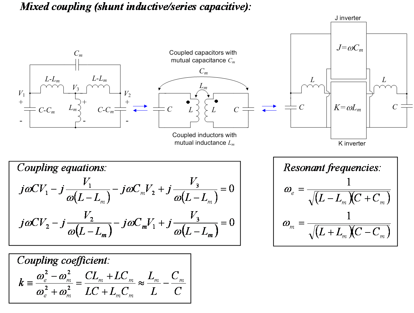
The basic coupling mechanisms between synchronously tuned pairs of resonators are summarized below. For each type of coupling, we show the coupling equations, the even and odd resonant frequencies (denoted ωe and ωm, respectively), and the coupling coefficient - all in terms of the lumped element values.
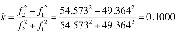
Suppose you had two coupled resonators and you wanted to know the value of the
coupling coefficient.
We can use Eq. (8) to extract the coupling coefficient
Figure 9 shows a Spice schematic with
two LC resonators inductively coupled. the coupling coefficient
 ,
,
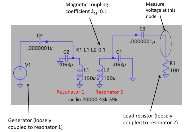
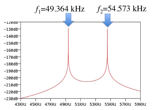
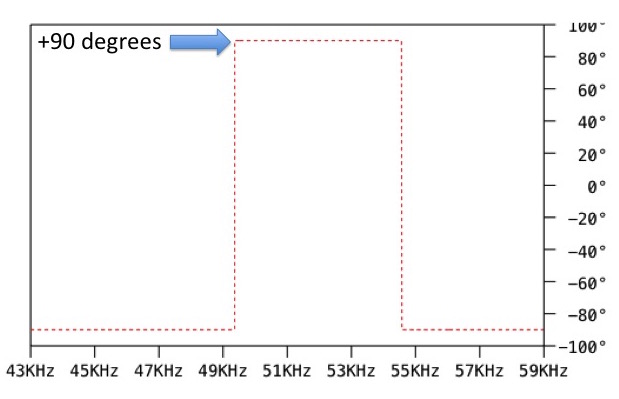
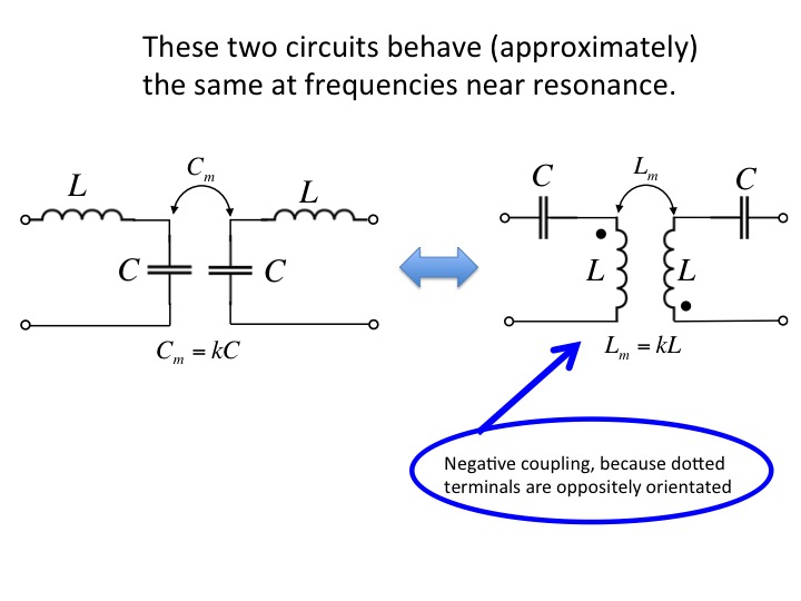
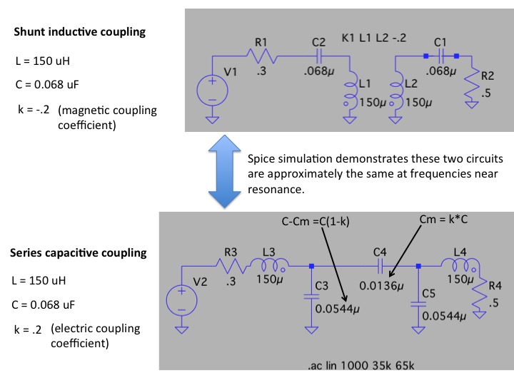
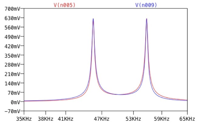
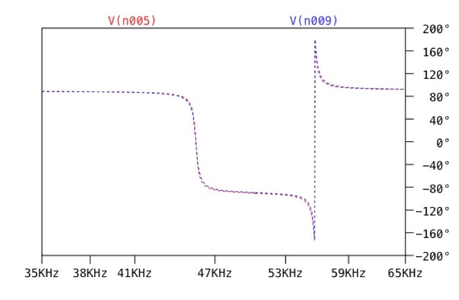
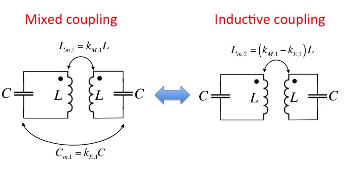
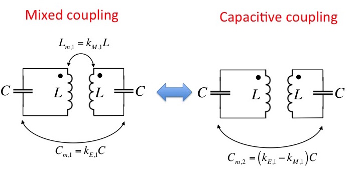
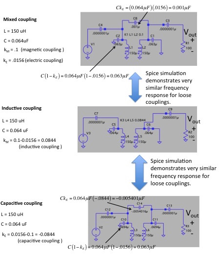
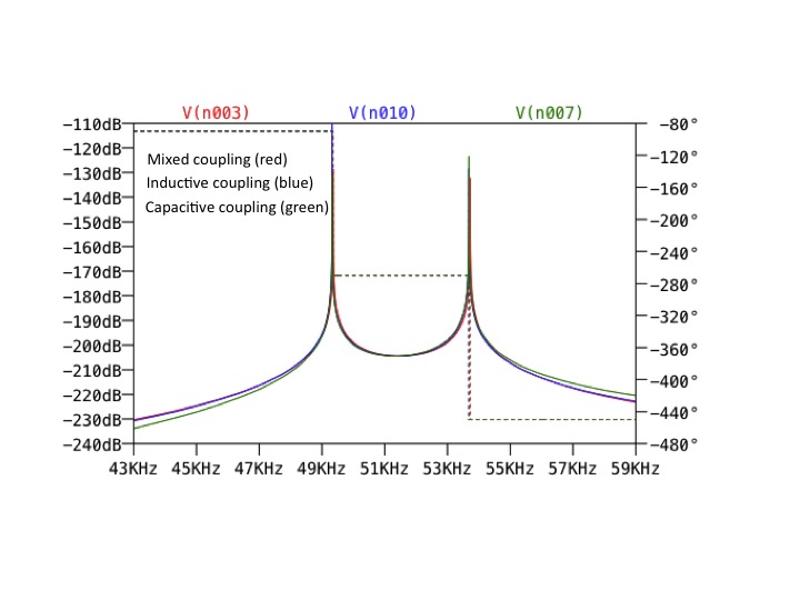
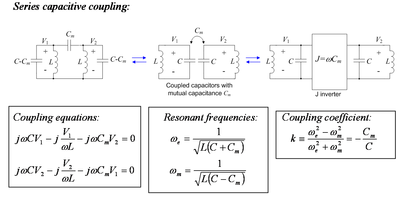
Or is it positive? Some people refer to electric (aka "series capacitive") as "negative" coupling. To get a better understanding of this, refer to Figure 12. Here we see that two LC resonant circuits capacitively coupled are equal to two LC resonant circuits inductively coupled with a negative mutual inductance (here we consider the mutual inductance are negative because the "dotted" terminals are on opposite sides.) We say these two circuits are equivalent in the sense that they both have the same eigenfrequencies (resonant frequencies) and almost identical phase response near resonance. Figure 13 shows a Spice schematic and simulation to illustrate how well this equality holds in a typical situation. The sign of coupling is rather relative. It's similar to how we assign an electron as being "negatively" charged. Notice how the phase in Figure 14 is -90 degrees between the resonant peaks. This "gives away" the sign of the coupling as negative. If the phase was +90 degrees then the sign of coupling would be considered "positive". Some people reverse what is positive and negative. Luckily, it makes no difference so long as a convention is established and you stick with that convention.